
Most everyday analysis is not modeling at all. You keep the columns you care about, keep the rows that match your question, and put the important ones on top. In SQL, the database language many analysts use, those three jobs are called SELECT, WHERE, and ORDER BY. In pandas, the Python table library, the same jobs are done with column lists, true/false filters, and sort_values. It is the same job spelled differently. Once you see the map, the fear drops.
The previous post in this Python for analytics series made DataFrames (pandas tables) feel like ordinary spreadsheets. This one shows how to slice them with clear patterns instead of clever one-liners that nobody can debug late on a Friday. If you already think in SQL from the SQL tutorials, you are ahead of the game. The habit of asking the right question first still applies, and it is covered in analytics foundations. The Learn page lists every series in order.
The mental model: filter, then pick columns, then sort
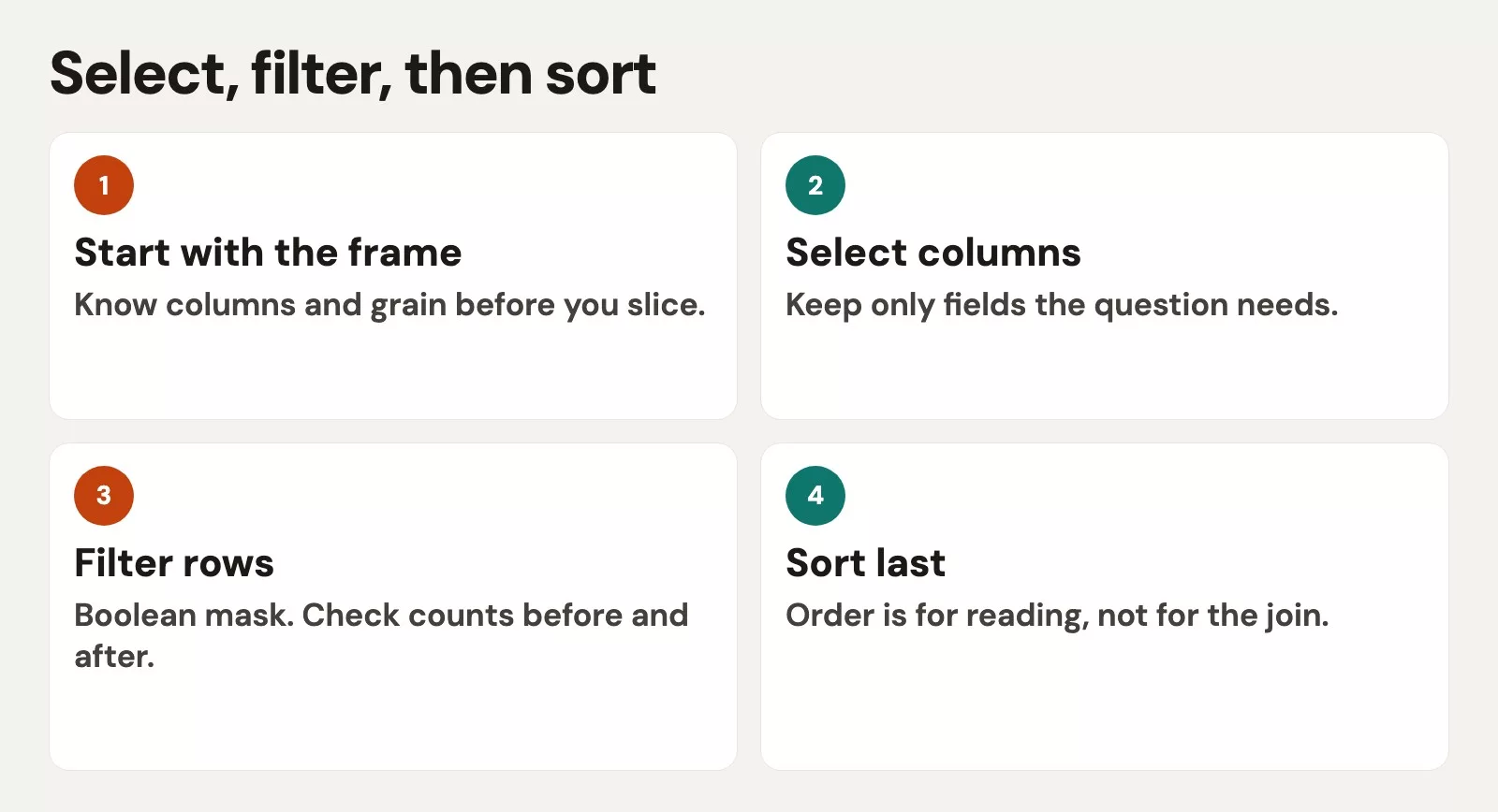
A SQL database decides for itself in what order to do the work, but people usually think in a fixed order: start from a table, filter the rows, pick the columns, and sort. A pattern that stays clear in pandas follows that same order:
- Filter the rows with a condition that returns True or False for each row.
- Select only the columns you need for the question.
- Sort the result so the rows read well.
You can reorder those steps if you need to, but teaching them in this order matches how a request usually sounds when a manager says it aloud: “East region only, show order id and revenue, highest first.”
SQL to pandas cheatsheet
| SQL idea | pandas pattern | Notes |
|---|---|---|
SELECT a, b | df[["a", "b"]] | Double brackets return a DataFrame |
SELECT a | df["a"] or df[["a"]] | Single brackets often return a Series |
WHERE x = 1 | df[df["x"] == 1] | Boolean mask inside brackets |
WHERE x > 10 AND y = 'East' | df[(df["x"] > 10) & (df["y"] == "East")] | Use & | with parentheses |
WHERE x IN (...) | df[df["x"].isin([...])] | Great for region lists |
WHERE x IS NULL | df[df["x"].isna()] | The later post on missing values goes deeper |
ORDER BY a DESC | df.sort_values("a", ascending=False) | Stable and readable |
ORDER BY a, b | df.sort_values(["a", "b"]) | List of columns |
LIMIT 10 | df.head(10) after sort | Or .iloc[:10] if needed |
SELECT DISTINCT a | df["a"].drop_duplicates() | Or df.drop_duplicates(subset=["a"]) |
Keep this table open in a tab. Most weekly work lives somewhere inside it.
Selecting columns
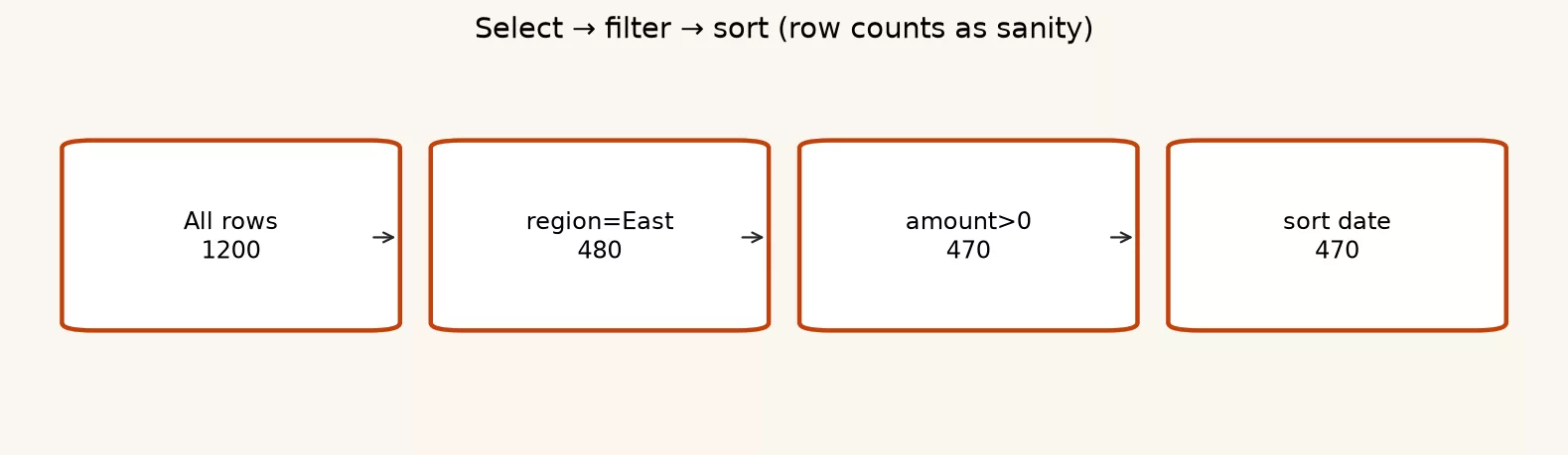
Keep a running count of rows as you filter, so you can see how each step narrows the table:
Start with the sample orders table from the earlier posts, or with any tidy table of your own, where each row is one order and each column is one field.
import pandas as pd

orders = pd.read_csv("hello_orders.csv")

# One column as a Series
regions = orders["region"]

# Several columns as a DataFrame (note the double brackets)
slim = orders[["order_id", "region", "revenue"]]

print(slim.head())
Double brackets feel odd until they become habit. A single column name gives back a Series, which is one column on its own, while a list of names gives back a DataFrame, which is a small table. If you need a one-column DataFrame on purpose, so you can keep using table methods, write [["revenue"]].
Selecting columns is also how you drop noise early. Wide exports with forty unused fields slow down reading and invite wrong joins later, so keep only what the question needs.
Filtering rows with boolean masks
A boolean mask is a column of True and False values, one for each row, that answers a yes-or-no question about that row. Put the mask inside brackets and pandas keeps only the rows marked True.
# Rows where region is East
east = orders[orders["region"] == "East"]

# Rows with revenue over 5000
big = orders[orders["revenue"] > 5000]

print(east)
print(big)
Example output:
| order_id | region | revenue | order_date |
|---|---|---|---|
| 1 | East | 1200 | 2026-01-03 |
| 3 | East | 5400 | 2026-01-04 |
You can combine conditions with & (and), | (or), and ~ (not). Always wrap each comparison in parentheses, because without them Python groups the pieces in the wrong order.
east_big = orders[
    (orders["region"] == "East") & (orders["revenue"] > 5000)
]

west_or_south = orders[orders["region"].isin(["West", "South"])]

print(east_big)
print(west_or_south)
Example:
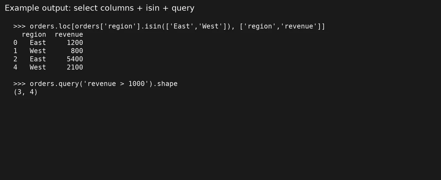
You may wonder why plain English and and or do not work here. Those words try to boil a whole column down to one True or False, while pandas needs to judge every row separately. The symbols and parentheses look a little mathy, but they are simply the dialect pandas speaks.
When the logic gets long, give each mask its own name so the last line reads like a sentence:
is_east = orders["region"] == "East"
is_big = orders["revenue"] > 5000
east_big = orders[is_east & is_big]
Named masks are kinder to reviewers, including you next month, than one deeply nested line.
Sorting
Sorting does not change what the data means. It only changes how the rows are presented, and therefore which rows you see first when you ask for the top of the table with head.
by_revenue = orders.sort_values("revenue", ascending=False)

by_region_then_revenue = orders.sort_values(
    ["region", "revenue"], ascending=[True, False]
)

print(by_revenue)
print(by_region_then_revenue)
Example output:
| order_id | region | revenue | order_date |
|---|---|---|---|
| 3 | East | 5400 | 2026-01-04 |
| 5 | West | 2100 | 2026-01-05 |
| 1 | East | 1200 | 2026-01-03 |
| 2 | West | 800 | 2026-01-03 |
| 4 | North | 300 | 2026-01-05 |
After a descending sort, head(3) gives you the top three by revenue, which is a common slide request. Ties can happen. If leadership cares about a stable ranking, add tie-breakers as extra sort columns so the order is the same every time.
loc and iloc, lightly
You will see loc and iloc everywhere online, and the short version is simple:
locselects by label, meaning the row labels and column names, which is useful when you want “rows where this is true, and only columns A and B” in one step.ilocselects by position, such as row 0 and column 1, which suits positional slices but not business rules about region names.
# Same filter + column project with loc
east_ids = orders.loc[orders["region"] == "East", ["order_id", "revenue"]]

# First three rows, first two columns by position
corner = orders.iloc[:3, :2]

print(east_ids)
print(corner)
For most analytics work, df[mask][columns] or a careful loc is enough. There is no prize for obscure indexing tricks, and the clear version is the one your team can review. Clarity ships.
Chaining carefully
Chaining means stacking several operations into one expression. It can read like an assembly line, but it turns into a debugging headache when you cannot see what any single step produced.
# Clear chain: parentheses let you break lines
result = (
    orders.loc[orders["revenue"] > 3000, ["order_id", "region", "revenue"]]
    .sort_values("revenue", ascending=False)
    .reset_index(drop=True)
)

print(result)
The call reset_index(drop=True) renumbers the rows from 0 again after filtering, which is tidy before you export. When you are still learning, or when a step deserves a comment about a business rule such as “exclude the internal test region,” prefer named intermediate variables.
# Same logic, easier to debug
active = orders[orders["revenue"] > 3000]
slim = active[["order_id", "region", "revenue"]]
result = slim.sort_values("revenue", ascending=False).reset_index(drop=True)
Both versions are professional, but the second is kinder when a reviewer asks what step two does, because you can point to a named line and print it.
Worked example: from full table to answer
Here is the business request: “Show West and East orders over $4,000, with only the id, region, and revenue, and put the highest revenue first.”
| order_id | region | revenue |
|---|---|---|
| 1 | East | 4200 |
| 2 | West | 8100 |
| 3 | East | 6900 |
| 4 | South | 1500 |
| 5 | West | 3200 |
import pandas as pd

orders = pd.read_csv("hello_orders.csv")

answer = (
    orders[
        orders["region"].isin(["East", "West"])
        & (orders["revenue"] > 4000)
    ][["order_id", "region", "revenue"]]
    .sort_values("revenue", ascending=False)
    .reset_index(drop=True)
)

print(answer)
The expected rows are order 2 (West, 8100), order 3 (East, 6900), and order 1 (East, 4200). South is left out because of its region, and the West order of 3200 is left out because it falls under the threshold. That is the whole game. Filter the rows, pick the columns, then sort.
Here is the same request written in SQL, so you can compare the two side by side:
SELECT
  order_id,
  region,
  revenue
FROM orders
WHERE region IN ('East', 'West')
  AND revenue > 4000
ORDER BY revenue DESC;
If your data already lives in a warehouse, meaning a company database built for reporting, prefer this SQL and skip the download. If you already have a file on your computer, the pandas version is the right tool, as the first post in this series explained.
Empty results are information
When a filter returns zero rows, do not assume the business has no matching activity. Check the boring causes first, because they are far more common than a real gap:
- Capital letters or spelling that differ, such as
EastversusEAST - Extra spaces hiding inside category labels
- Threshold units that do not match, such as dollars versus thousands of dollars
- Date filters applied to a column that is still stored as plain text
- A table that you filtered twice by accident
# Quick diagnostics when a filter looks "too empty"
print(orders["region"].unique())
print(orders["revenue"].min(), orders["revenue"].max())
print(orders.shape)
print(orders[orders["region"] == "East"].shape)
Print the unique values and the smallest and largest numbers before you rewrite the whole notebook (a document that mixes code, results, and notes). Most “pandas is broken” moments turn out to be “my assumption about the data was wrong,” which is normal analytics work and not a personal failure.
The same diagnostic habit applies when a filter returns too many rows. If you expected dozens and got tens of thousands, you may have used | where you meant &, or forgotten parentheses, so the filter did not mean what you read in English.
Making a safe copy before you change a slice
You may see a warning called SettingWithCopy when you filter a table and then change values inside the slice. pandas cannot tell whether you meant the original or only the slice. A safe habit is to make your intention obvious whenever you want a standalone table.
east = orders.loc[orders["region"] == "East"].copy()
east["revenue_k"] = east["revenue"] / 1000
Adding .copy() tells pandas that this is your new working table, so you avoid accidental links back to the parent table. The later post on pipelines leans on clear assignments like this one.
Common mistakes
- Using the Python words
andandorbetween conditions. Use the symbols&and|with parentheses around each condition instead. - Forgetting that one column pulled out with single brackets is a Series. Some methods behave slightly differently on a Series than on a DataFrame, so check what you have before you call them.
- Filtering at the wrong level of detail. If each row is a customer and you apply a rule meant for individual orders, you get nonsense.
- Sorting for a “top few” list and then forgetting the filter. The order of your steps should match the business sentence, or the top rows may not be the ones the question asked for.
- Matching text that differs only by capital letters. To pandas,
"east"is not the same as"East", so clean up the categories first when your sources are messy. - Chaining so much that nobody can slip in a row count check. Print the table’s
shape, which is its row and column count, after any big filter. - Using positions for business rules. Row positions shift whenever the data changes, so write the rule as a condition on a column instead of relying on
iloc.
Rule of thumb: Write the request as “which rows, which columns, which order,” and then build those three steps with a mask, a column list, and
sort_values.
Quick recap
- A list of column names does the job of SELECT, which is choosing what to keep.
- A boolean mask does the job of WHERE, which is choosing which rows to keep, and it needs symbols and parentheses to combine conditions.
- The
sort_valuesmethod does the job of ORDER BY, which puts the rows in a useful order. - Use
locto pick rows and columns by label, and useiloconly when you truly mean a position. - Chain steps only while the result stays readable, and otherwise give each step a name.
- Check the row count after each filter, so you know what you actually kept.
Practice and next step
Using your practice CSV file, a plain spreadsheet-style text file, or a real extract from your own data:
- Select just two columns and print the first few rows.
- Filter to one region and print the row count before and after, so you can see the effect.
- Combine that region filter with a numeric threshold, using parentheses.
- Sort from highest to lowest on the numeric column and show the top three rows.
- Write the same logic as SQL comments above your pandas code, to prove to yourself that the two match.
The next post covers grouping and totals. It maps GROUP BY to a split, calculate, and combine routine, so you can answer “total by region” without building a spreadsheet pivot table every time.
Sources
- pandas, “Indexing and selecting data”: https://pandas.pydata.org/docs/user_guide/indexing.html
- pandas
DataFrame.sort_values: https://pandas.pydata.org/docs/reference/api/pandas.DataFrame.sort_values.html - pandas
Series.isin: https://pandas.pydata.org/docs/reference/api/pandas.Series.isin.html - pandas, “10 minutes to pandas”: https://pandas.pydata.org/docs/user_guide/10min.html
- Analytics Made Simple, Learn: https://analyticsmadesimple.com/learn/
- Analytics Made Simple, SQL series: https://analyticsmadesimple.com/series/sql/
- Analytics Made Simple, Analytics foundations: https://analyticsmadesimple.com/series/analytics-foundations/
- Analytics Made Simple, From spreadsheets to real data: https://analyticsmadesimple.com/series/spreadsheets-to-data/
Keep going
Same lessons in your feed
Short diagrams, hooks, and weekly tutorials on Substack, Instagram, X, and Facebook.