DataFrames as tables

If Python for analytics clicked for anyone, it was usually the day they realized a DataFrame is not a new religion. It is a table: rows that mean something, columns with names, and types that decide what math is allowed. Once you see that, the rest of pandas becomes vocabulary on top of a shape you already understand from Sheets and SQL.

This is Part 3 of Python for analytics. Part 2 got you a working environment. Now we treat DataFrames as tables you can inspect with confidence. If grain and tidy structure are still fuzzy, revisit From spreadsheets to real data and the problem framing in Analytics foundations. SQL table instincts from the SQL series transfer almost one-to-one.

What you will learn

• What a DataFrame is in plain language (and what a Series is)
• How rows, columns, and dtypes map to sheets and SQL
• How to load a CSV and inspect it with head, shape, columns, info, and dtypes
• What the index is (lightly) and when to ignore it for now
• How to rename columns without creating silent chaos
• A worked example you can rerun on any tidy CSV

DataFrame in one paragraph

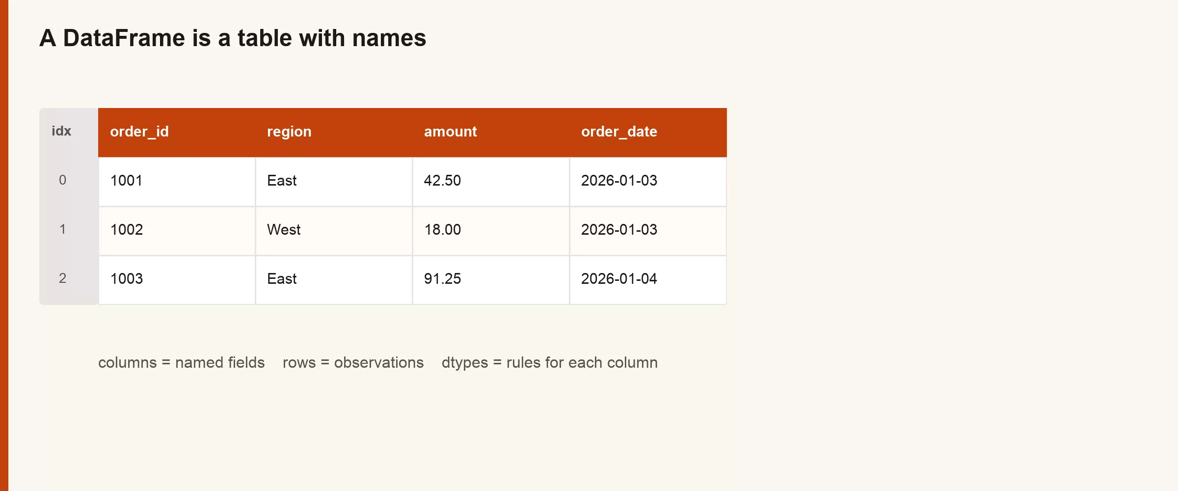
What a small DataFrame looks like as a table:

A DataFrame is a two-dimensional table with labeled columns. Each column is a Series: a single named list of values with a shared type when possible. One row is one observation at a chosen grain (one order, one customer-day, one ticket). That is the same mental model as a well-built sheet range or a SQL table. pandas adds programming: assign the table to a variable, transform it, and keep the steps in code instead of in fragile click history.

You will also meet the index: labels for rows. By default, reading a CSV gives you 0, 1, 2, … which is fine. Later you might set an order id as the index. For learning filters and groupbys, treating the index as “row labels in the background” is enough. Do not let index mystique block you from loading a file.

Spreadsheet idea to DataFrame idea

Translation table for people who think in grids first:

Notice what is missing: merged cells, colors as data, and “notes in column Z.” Those sheet habits do not map cleanly. Tidy rectangular data maps cleanly. If your export has two header rows and a title in A1, clean that in the source export or with explicit skip logic. Part 8 will pipeline the mess. Part 3 assumes a simple header.

Load a CSV the way professionals start

Most analytics Python sessions begin with a read. Keep the sample from Part 2 or any tidy CSV.

import pandas as pd

orders = pd.read_csv("hello_orders.csv")

print(orders.head())
print("shape:", orders.shape)
print("columns:", orders.columns.tolist())

Example output:

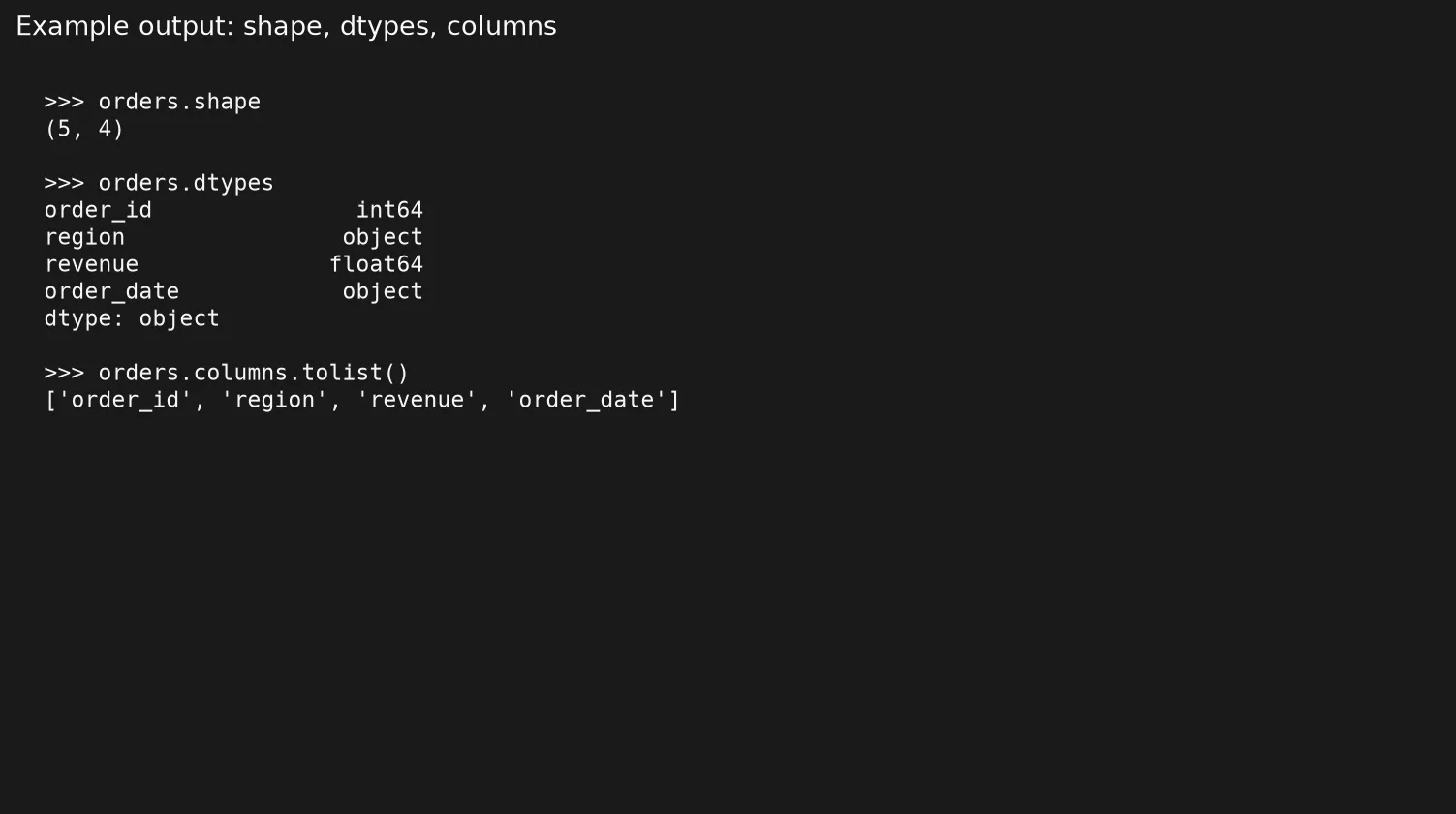
head() shows the first five rows by default. Pass a number for more or less: head(10). shape returns (rows, columns). That tuple is your first sanity check: if you expected 5,000 orders and shape says 50, something went wrong upstream, not in the pivot.

Always look at column names early. Spaces, weird capitalization, and accidental units in the header (“Revenue (USD)”) become annoying later. Renaming is cheap. Living with bad names for twenty steps is expensive.

dtypes: the quiet rulebook

A dtype is the data type of a column: integer, float, string-like object, boolean, datetime, and others. Types decide whether sum makes sense, whether a join key matches, and whether “2024-01-01” is a date or a pile of text.

print(orders.dtypes)
print(orders.info())

info() is a quick medical chart: column names, non-null counts, dtypes, and memory use. If a revenue column is object (often “string-ish”) because of a stray dollar sign or comma, sums will misbehave. Part 7 goes deep on casting and missing values. For now, train your eyes: after every load, glance at dtypes before you trust a total.

Common first-day mappings:

• Counts and ids that never need decimals: integers when clean
• Money and rates: floats (with the usual float caveats; finance systems may use decimals later)
• Categories like region: strings (pandas may show object or string)
• Dates: ideally datetime, not free text

If SQL is your home language, dtypes are cousins of column types in CREATE TABLE. The names differ. The discipline is the same: types are part of the contract, not an afterthought.

Rows mean grain; columns mean attributes

Before fancy methods, write one sentence: one row means _____. For hello_orders.csv, one row means one order. If you later group to region totals, one row will mean one region. Shape changes with grain. That is normal. Confusion starts when you mix grains without noticing.

Columns are attributes of that grain: identifiers, dimensions (region), facts (revenue). This is the same vocabulary you use in warehouse modeling, just lighter. If a column does not describe the row grain, you may have a layout problem (a wide sheet that should be tall) or a join residue. Spotting that early is analytics maturity, not pedantry.

Rename columns without drama

Readable names make every later line cheaper. Prefer snake_case for code friendliness: order_id, region, revenue.

orders = orders.rename(
    columns={
        "order_id": "order_id",  # already good; shown for pattern
        "region": "region",
        "revenue": "revenue_usd",
    }
)

# Or rename many messy headers at once after a bad export:
# orders.columns = ["order_id", "region", "revenue_usd"]

print(orders.head())
print(orders.dtypes)

Example:

Example output:

Two styles exist: dictionary rename when you only fix a few labels, and assigning a full list to columns when the export order is fixed and names are hopeless. Dictionary rename is safer when columns might reorder. Full list assignment is faster when you control the file contract.

Assign back to orders (or use inplace carefully). Beginners often call rename and wonder why nothing changed: they forgot to keep the returned DataFrame. pandas methods frequently return a new object. That is a feature for safe pipelines, not a trick.

Worked example: inspect, then tidy names

Imagine a slightly messier export (still rectangular):

Order ID,Region Name,Revenue USD
1,East,4200
2,West,8100
3,East,6900
4,South,1500
5,West,3200

Full inspection pattern you can reuse at work:

import pandas as pd

path = "hello_orders_messy_headers.csv"
orders = pd.read_csv(path)

print("=== head ===")
print(orders.head())

print("=== shape ===")
print(orders.shape)

print("=== columns ===")
print(orders.columns.tolist())

print("=== dtypes ===")
print(orders.dtypes)

print("=== info ===")
orders.info()

orders = orders.rename(
    columns={
        "Order ID": "order_id",
        "Region Name": "region",
        "Revenue USD": "revenue_usd",
    }
)

print("=== after rename ===")
print(orders.head())
print(orders.dtypes)

Expected story: five rows, three columns, integer revenue if the file is clean, and human-friendly snake_case names afterward. If Revenue USD imported as text, info() will show it. Do not average a text column and blame pandas. Fix the type (Part 7) or fix the export.

Mini result table after rename:

Series vs DataFrame without the identity crisis

New learners lose time wondering why a method “disappeared.” Often they hold a Series when they thought they held a DataFrame.

col = orders["revenue"]          # Series
tab = orders[["revenue"]]        # DataFrame with one column
print(type(col), type(tab))
print(col.mean())
print(tab.mean())  # still works; result shape differs

A Series is closer to a single SQL column result. A DataFrame is closer to a table. Many operations exist on both, but selection rules differ, and some table-oriented helpers expect two dimensions. When an error mentions Series, check whether you used single brackets by accident.

You do not need to memorize the entire class hierarchy. You need a reflex: when confused, print type(...), shape if it exists, and head. Those three prints solve more early bugs than rereading a chapter.

Index, lightly

Print orders.index and you will see a RangeIndex starting at 0. That is normal. Some tutorials immediately set a meaningful index. You can wait. Filtering with clear column conditions (Part 4) is easier to read for SQL-minded people than clever index tricks.

When might you care sooner?

• Time series labeled by date
• Joins that accidentally duplicate index labels
• Alignment behavior when combining Series

For Part 3, remember: columns are your main handles. Index is row labels. If a method returns something that “looks like a table but weird,” check whether you are holding a Series, a DataFrame, or a GroupBy object (Part 5).

Peek at values without drowning

Beyond head, a few cheap peeks help you learn a table’s personality before you transform it.

print(orders.tail(3))          # last rows; useful for time-sorted files
print(orders.sample(3, random_state=1))  # random peek; set seed for reuse
print(orders["region"].value_counts())   # category frequencies
print(orders["revenue"].describe())      # numeric summary

value_counts is the quick “what is in this column?” tool. If you expected three regions and see twelve spellings of East, you found a cleaning job early. describe on a numeric column gives count, mean, min, max, and quartiles. It is not a full statistical report. It is a flashlight.

When a column should be numeric but describe fails or looks empty of real stats, check dtypes again. Text that looks like numbers is still text until you cast it. That theme returns hard in Part 7. For Part 3, the skill is noticing the mismatch without panic.

One more habit: compare len(orders) with orders.shape[0]. They should match. If you ever filter and assign wrong, these checks catch empty frames before you email a blank summary. Empty is a valid intermediate result. Silent empty is how weekends get ruined.

How this connects to SQL and Sheets day to day

In Sheets, you stare at the grid. In SQL, you SELECT * with a LIMIT. In pandas, head() is that limit, and info() is a quick DESCRIBE-like glance (not identical to SQL DESCRIBE, but same spirit: what am I holding?).

Professional habit across all three tools: profile before you transform. Count rows. List columns. Check types. Spot nulls. Only then filter, join, or aggregate. People who skip profiling ship confident wrong dashboards. People who profile look slower for five minutes and faster for the rest of the week.

Common mistakes

• Assuming the CSV is tidy because it opens in Excel. Two header rows and blank spacer columns still “open.”
• Never checking shape. You filter wrong and analyze 12 rows thinking you have 12,000.
• Ignoring dtypes until a sum looks insane. Make dtypes a reflex after read_csv.
• Spaces in column names without a plan. df["Revenue USD"] works, but it is annoying. Rename early.
• Thinking the index is “the data.” Usually your keys should be real columns until you have a reason.
• Calling rename and discarding the result. Keep the returned frame.
• Mixing grains in one frame without labeling. Order rows and region totals are different tables.

Rule of thumb: After every load, run head, shape, and dtypes (or info) before you calculate anything you would put in a slide.

Practice and next step

Take any small tidy CSV you own (or the hello file) and write a short “table card” in comments or a note:

• One row means…
• Primary key candidate (if any)…
• Column list and dtypes…
• Anything surprising in head()…

Then rename at least one column to a clearer name and reprint head().

Next: Part 4, Selecting, filtering, sorting, maps SQL SELECT / WHERE / ORDER BY onto clear pandas patterns without cleverness for its own sake.

Quick recap

• A DataFrame is a labeled table; a Series is one column.
• Map sheet headers and SQL columns to columns, shape, and dtypes.
• Start sessions with read_csv, then head, shape, info/dtypes.
• Say the grain out loud: one row means…
• Rename early; keep returned objects.
• Treat the index lightly until you need it.

Sources

• pandas, “Intro to data structures”: https://pandas.pydata.org/docs/user_guide/dsintro.html
• pandas, “10 minutes to pandas”: https://pandas.pydata.org/docs/user_guide/10min.html
• pandas read_csv: https://pandas.pydata.org/docs/reference/api/pandas.read_csv.html
• pandas DataFrame.rename: https://pandas.pydata.org/docs/reference/api/pandas.DataFrame.rename.html
• Analytics Made Simple, Learn: https://analyticsmadesimple.com/learn/
• Analytics Made Simple, Analytics foundations: https://analyticsmadesimple.com/series/analytics-foundations/
• Analytics Made Simple, From spreadsheets to real data: https://analyticsmadesimple.com/series/spreadsheets-to-data/
• Analytics Made Simple, SQL series: https://analyticsmadesimple.com/series/sql/

Merch on Etsy

Open store →

Naive Bayes T-Shirt View on Etsy → Apache Flink Shirt View on Etsy → Apache Kafka T-Shirt View on Etsy → Y-Hat Coffee Mug View on Etsy →