
To turn a long list of rows into a short summary, such as total sales for each region, group the rows and then add, average, or count them. In a spreadsheet that is a pivot table, and in pandas, the popular Python library for tables, it is groupby followed by a calculation. Say you have thousands of order rows and your manager wants one small table of region totals. The idea is the same in every tool, and so are the risks, such as counting at the wrong level or double-counting duplicate rows.
This post continues the Python for analytics series, picking up right after the posts that loaded and sliced tables. Now we summarize them. If you already write SQL (the standard language for asking a database for data) aggregates, you will feel at home here. If you live in pivot tables, you will recognize the move too. Keep your SQL and spreadsheet habits nearby, along with the problem discipline from Analytics foundations. Charts can wait; a later post in this series can plot what you group here, once the numbers themselves are right.
Split, apply, combine
Hadley Wickham popularized a simple name for what group-by does in many tools: split the table into groups, apply a function to each group (sum, mean, count), then combine the results into a new table. pandas groupby is that engine, and you do not need the academic history to use it well. You just need the picture:
- Split on region: East rows together, West rows together, South rows together.
- Apply sum to revenue inside each pile.
- Combine into a small table with one row per region.
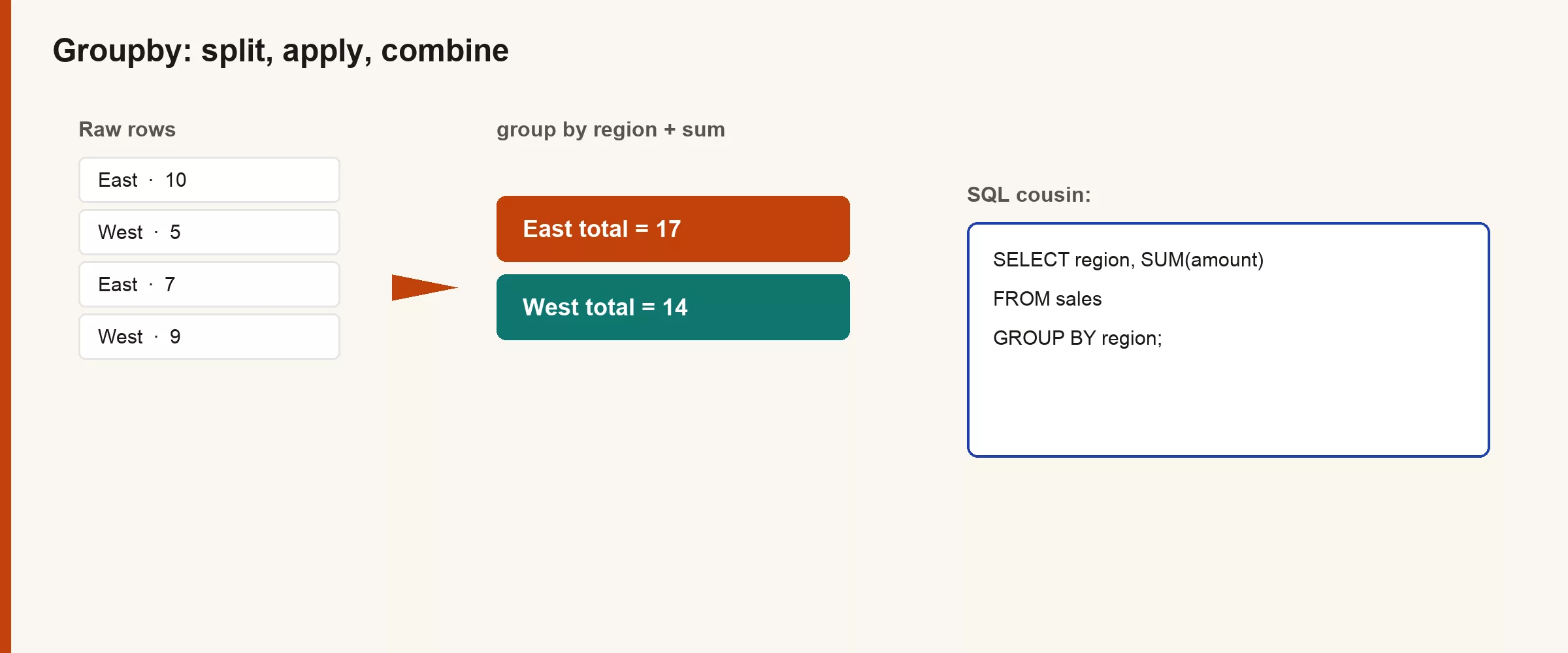
The grain changes on purpose here: before, you had one row per order, and after, you have one row per region. If you forget that shift, you will join the summary back to the detail rows incorrectly and inflate your totals. Say the new grain out loud every time you group, even if it feels obvious in the moment.
SQL mind to pandas mind
| SQL | pandas |
|---|---|
SUM(revenue) | .sum() on a grouped column |
AVG(revenue) | .mean() |
COUNT(*) | .size() or .count() (see notes below) |
COUNT(DISTINCT x) | .nunique() |
GROUP BY region | groupby("region") |
GROUP BY region, channel | groupby(["region", "channel"]) |
| Multiple metrics in one SELECT | .agg(...) with a dict or named aggregation |
One pair in that table is worth slowing down on: count in pandas counts non-null values per column, while size counts rows in the group, including rows where some columns are null. For “how many orders,” size (or counting a never-null id column) is usually closer to SQL’s COUNT(*).
First aggregations: sum, mean, count
Using the familiar orders file:
import pandas as pd

orders = pd.read_csv("hello_orders.csv")

# Total revenue by region (Series indexed by region)
totals = orders.groupby("region")["revenue"].sum()
print(totals)

# Same idea as a DataFrame with a normal region column
totals_df = (
    orders.groupby("region", as_index=False)["revenue"]
    .sum()
    .rename(columns={"revenue": "total_revenue"})
)
print(totals_df)

# Average order size by region
avg_df = (
    orders.groupby("region", as_index=False)["revenue"]
    .mean()
    .rename(columns={"revenue": "avg_revenue"})
)
print(avg_df)

# Number of orders by region
counts = orders.groupby("region").size().reset_index(name="order_count")
print(counts)
Example output:
| region | total_revenue | n_orders |
|---|---|---|
| East | 6600 | 2 |
| West | 2900 | 2 |
| North | 300 | 1 |
as_index=False keeps the group keys as normal columns, which is usually what you want before you export to CSV (a plain spreadsheet-style text file) or join back to something else. If you forget it, running reset_index() after the aggregation is the standard repair.
Multiple aggregations with agg
Real questions rarely want only a sum. They usually want sum and count and maybe average, all in one table, so you are not stitching three separate results together by hand.
summary = (
    orders.groupby("region", as_index=False)
    .agg(
        total_revenue=("revenue", "sum"),
        avg_revenue=("revenue", "mean"),
        order_count=("order_id", "count"),
    )
    .sort_values("total_revenue", ascending=False)
)

print(summary)
Example:
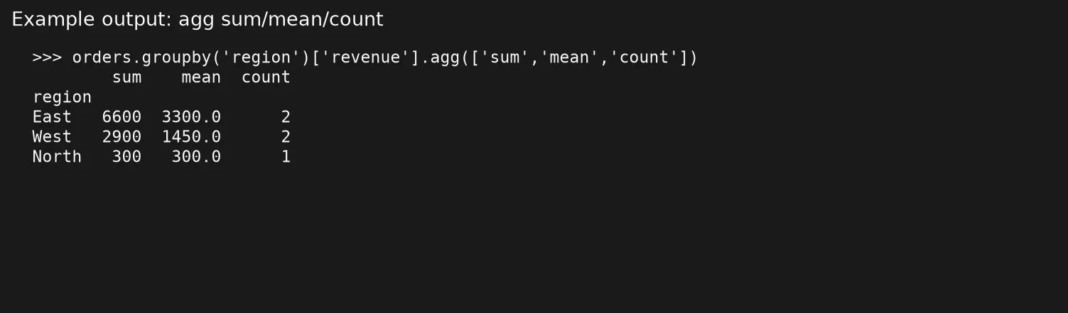
Named aggregation, the new_name=("column", "function") style above, keeps your column names readable. Older code uses nested dictionaries instead, and you may still run into that style online, but prefer named aggregation when you can, because it reads clearly in code review.
You can also aggregate different columns differently:
# If you had more columns, e.g. quantity and revenue:
# orders.groupby("region", as_index=False).agg(
#     total_revenue=("revenue", "sum"),
#     total_units=("quantity", "sum"),
#     orders=("order_id", "nunique"),
# )
Worked example: sales by region before and after
Visual: row-level data vs groupby total:
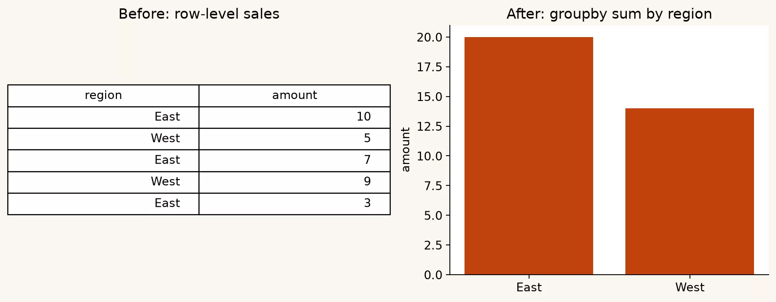
Before (order grain):
| order_id | region | revenue |
|---|---|---|
| 1 | East | 4200 |
| 2 | West | 8100 |
| 3 | East | 6900 |
| 4 | South | 1500 |
| 5 | West | 3200 |
After (region grain):
| region | total_revenue | avg_revenue | order_count |
|---|---|---|---|
| West | 11300 | 5650 | 2 |
| East | 11100 | 5550 | 2 |
| South | 1500 | 1500 | 1 |
import pandas as pd

orders = pd.DataFrame(
    {
        "order_id": [1, 2, 3, 4, 5],
        "region": ["East", "West", "East", "South", "West"],
        "revenue": [4200, 8100, 6900, 1500, 3200],
    }
)

by_region = (
    orders.groupby("region", as_index=False)
    .agg(
        total_revenue=("revenue", "sum"),
        avg_revenue=("revenue", "mean"),
        order_count=("order_id", "count"),
    )
    .sort_values("total_revenue", ascending=False)
    .reset_index(drop=True)
)

print(by_region)

# Optional: share of total revenue
by_region["pct_of_total"] = (
    by_region["total_revenue"] / by_region["total_revenue"].sum()
)
print(by_region)
That pct_of_total column is a common slide request, and it is worth noticing that it is calculated on the aggregated table, not by averaging percentages at the order level. Percent of total is a post-aggregation story. Mixing levels is exactly how people end up with “math that does not add to 100%,” and then have to argue about it in a meeting.
Equivalent SQL:
SELECT
  region,
  SUM(revenue) AS total_revenue,
  AVG(revenue) AS avg_revenue,
  COUNT(*) AS order_count
FROM orders
GROUP BY region
ORDER BY total_revenue DESC;
This SQL does the same as the pandas groupby above: for each region it adds up revenue, averages it, and counts orders, then lists the regions from highest total to lowest. Seeing both versions side by side shows that the grouping idea is the same in either tool.
Grouping by more than one column
Multi-key groups are normal: region and month, team and status, product and channel. Pass a list to groupby and it handles the rest.
# Toy extension: add a channel column
orders["channel"] = ["web", "web", "store", "web", "store"]

by_region_channel = (
    orders.groupby(["region", "channel"], as_index=False)
    .agg(
        total_revenue=("revenue", "sum"),
        order_count=("order_id", "count"),
    )
    .sort_values(["region", "total_revenue"], ascending=[True, False])
)

print(by_region_channel)
Example:
| region | channel | total_revenue | n_orders |
|---|---|---|---|
| East | web | 6600 | 2 |
| East | store | 0 | 0 |
| West | web | 2100 | 1 |
| West | store | 800 | 1 |
Each unique pair becomes its own group, so the row counts in the summary should still match the sum of the group counts, as long as you are only counting. Verify that with a total row whenever the stakes are high enough to matter.
reset_index and the shape of the result
After a groupby, you might end up holding any of three shapes: a Series with a single metric and the group keys as its index, a DataFrame (a pandas table) with a MultiIndex where multiple group keys sit as index levels, or a flat DataFrame with the keys as ordinary columns, using as_index=False or reset_index().
For handoffs to Sheets, business intelligence tools, or teammates who would rather not deal with an index at all, prefer the flat DataFrame. A later post in this series cares specifically about export shapes, so it helps to start clean now.
s = orders.groupby("region")["revenue"].sum()
flat = s.reset_index(name="total_revenue")
print(flat)
Filter then group, or group then filter?
Both happen, and they answer genuinely different questions, so it pays to keep them straight.
- Filter then group: “Among web orders only, revenue by region.” Apply a row-level mask first, the same kind covered earlier in this series, and then run the groupby.
- Group then filter groups: “Regions with total revenue over 10,000.” Aggregate first, then filter the summary table, which is the same energy as SQL’s
HAVINGclause.
# HAVING-style filter on aggregates
strong_regions = by_region[by_region["total_revenue"] > 10000]
print(strong_regions)
Do not mix these up in a meeting, because “orders over $10k by region” is not the same claim as “regions over $10k total,” and swapping them changes the story you are telling.
Sanity checks that catch bad groupbys
Aggregation errors tend to be quiet ones. The code runs without complaint, the resulting number looks reasonably round, and someone puts it straight into a slide before anyone double-checks it. Build a short checklist into your muscle memory so that does not happen to you.
# 1) Detail total vs group totals for an additive metric
detail_total = orders["revenue"].sum()
group_total = by_region["total_revenue"].sum()
print(detail_total, group_total, detail_total == group_total)

# 2) Row counts
print(len(orders), by_region["order_count"].sum())

# 3) Unexpected group labels
print(by_region["region"].tolist())
If the detail total and the group total disagree, you likely filtered one side and not the other, or you aggregated a column that stopped being purely additive after a join exploded some rows. If the order counts disagree with len(orders), you may have dropped null keys from the group column, since pandas can exclude them from groups depending on version and settings. Glance at orders["region"].isna().sum() whenever a count looks short.
Also watch for grouping by a continuous number by accident. Grouping on revenue itself creates one group per distinct dollar amount, which is almost never the summary leadership actually wanted. Group by (summarize rows that share a value) dimensions, such as region, month, or segment, and aggregate facts, such as revenue or quantity, and keep those two roles separate in your head.
Charts are optional later
A grouped bar chart of total_revenue by region is the natural picture for this table, and this series does come back to plotting later, but treat that as a later stretch rather than a blocker now. Get the numbers right first, because a wrong chart with pretty colors is still a wrong chart. When you do plot, feed it the aggregated table rather than the raw orders, unless you specifically mean to show a distribution.
Common mistakes
- Averaging averages. The mean of several regional averages is not the same as the overall mean once regions differ in size.
- Grouping on a column with hidden duplicates or trailing spaces.
"East"and"East "become two separate groups, so clean the categories first. - Using
countwhen you meant a row count with nulls present. Know the difference betweencountandsizebefore you rely on either. - Forgetting the grain change. Joining region totals back onto order rows without care multiplies the totals instead of matching them.
- Summing an id column by accident. Aggregate the fact columns, not the key columns, unless you have a specific reason to.
- Silent wrong results from pre-aggregated inputs. If the CSV is already a pivot, grouping it again can double-count, so profile the file with
headand check what each row means before you trust it. - Skipping a totals check. The sum of the group totals should match the sum of the detail metric, for summable facts without filters in play.
Rule of thumb: After every groupby, write “one row now means…” and check that the sum of the group sums equals the ungrouped sum for additive metrics.
Practice this week
On your own practice data:
- Compute total revenue by region with
as_index=False. - Add order counts and average revenue with
agg, so each total comes with the context needed to read it. - Sort by total revenue descending.
- Filter the summary to groups above a threshold, the HAVING-style move.
- Verify that the group totals sum to the overall total revenue.
Once that feels routine, you are ready for the next stretch of this series, which brings a second table into the picture with the same grain caution you just practiced here, followed by a post on missing values and data types.
Quick recap
groupbyis split-apply-combine, and it changes the grain of your table on purpose.- Map SQL’s
SUM/AVG/COUNTandGROUP BYto pandas’sum/mean/count/sizeandgroupby. - Use
aggfor multiple metrics at once, and prefer named aggregations when you can. as_index=Falseorreset_indexkeeps your results flat and easy to hand off.- Filtering rows before you group answers a different question from filtering the group totals afterward, which SQL does with a HAVING clause (a filter that runs on the totals, after grouping).
- Charts are optional later; correct tables always come first.
Series notes
This post is part of the Python for analytics series. The posts before this one loaded and sliced tables; the next brings joins and merges into the picture, and the one after that covers missing values and data types.
Sources
- pandas, “Group by: split-apply-combine”: https://pandas.pydata.org/docs/user_guide/groupby.html
- pandas
DataFrame.groupby: https://pandas.pydata.org/docs/reference/api/pandas.DataFrame.groupby.html - pandas
DataFrame.agg: https://pandas.pydata.org/docs/reference/api/pandas.DataFrame.agg.html - pandas, “10 minutes to pandas”: https://pandas.pydata.org/docs/user_guide/10min.html
- Analytics Made Simple, Learn: https://analyticsmadesimple.com/learn/
- Analytics Made Simple, SQL series: https://analyticsmadesimple.com/series/sql/
- Analytics Made Simple, From spreadsheets to real data: https://analyticsmadesimple.com/series/spreadsheets-to-data/
- Analytics Made Simple, Analytics foundations: https://analyticsmadesimple.com/series/analytics-foundations/
Keep going
Same lessons in your feed
Short diagrams, hooks, and weekly tutorials on Substack, Instagram, X, and Facebook.