

Before you fix a messy table, you should look at it. That look is called profiling, and it means counting rows, checking what is blank, finding the smallest and largest values, and scanning the categories for odd spellings. Every cleaning step you take afterward then has a reason behind it.
Say a coworker sends you a CSV file (a plain table saved as text) and asks you to clean it before the executive review. You open it, see a few blank cells, and your hand goes to find-and-replace. That instinct is kind, but it is how you paint over a stain while the leak keeps running behind the wall. The earlier post in this series gave you five words for how data goes wrong. This one gives you the flashlight to find out which of them you actually have.
The examples stay hands-on. You get SQL you can run in a warehouse notebook, Python you can run with the pandas library, and a habit of never cleaning blind.
Why polishing first fails
Cleaning without a profile is like repainting a wall with a water stain. The screenshot may look better afterward, but you still do not know whether the leak comes from a blank-field policy, a broken join key, a late data feed, or five spellings of the same region. Each of those needs a different fix.
A profile answers a short list of questions. What is in the table, and how much of it is missing? What are the smallest and largest values? Which categories dominate, and which look like typos? How many rows claim to be unique when they are not? You are not building a forty-page data catalog. You are earning the right to change values, because you can now say what was wrong before you touched anything.
This pairs with habits from the series on moving from spreadsheets to real data, where you look before you reshape, and from the Python for analytics series, where you inspect a table before you group it. Data quality is the same discipline with trust as the output.
The lightweight profile checklist
Example profile output: null rates by column:
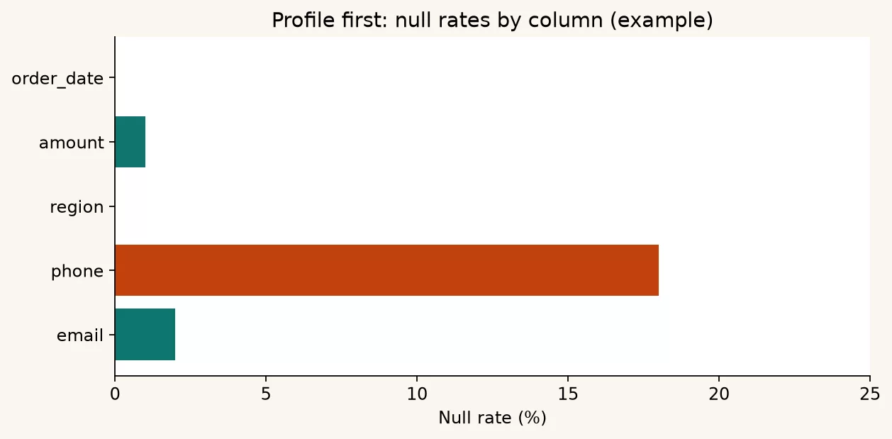
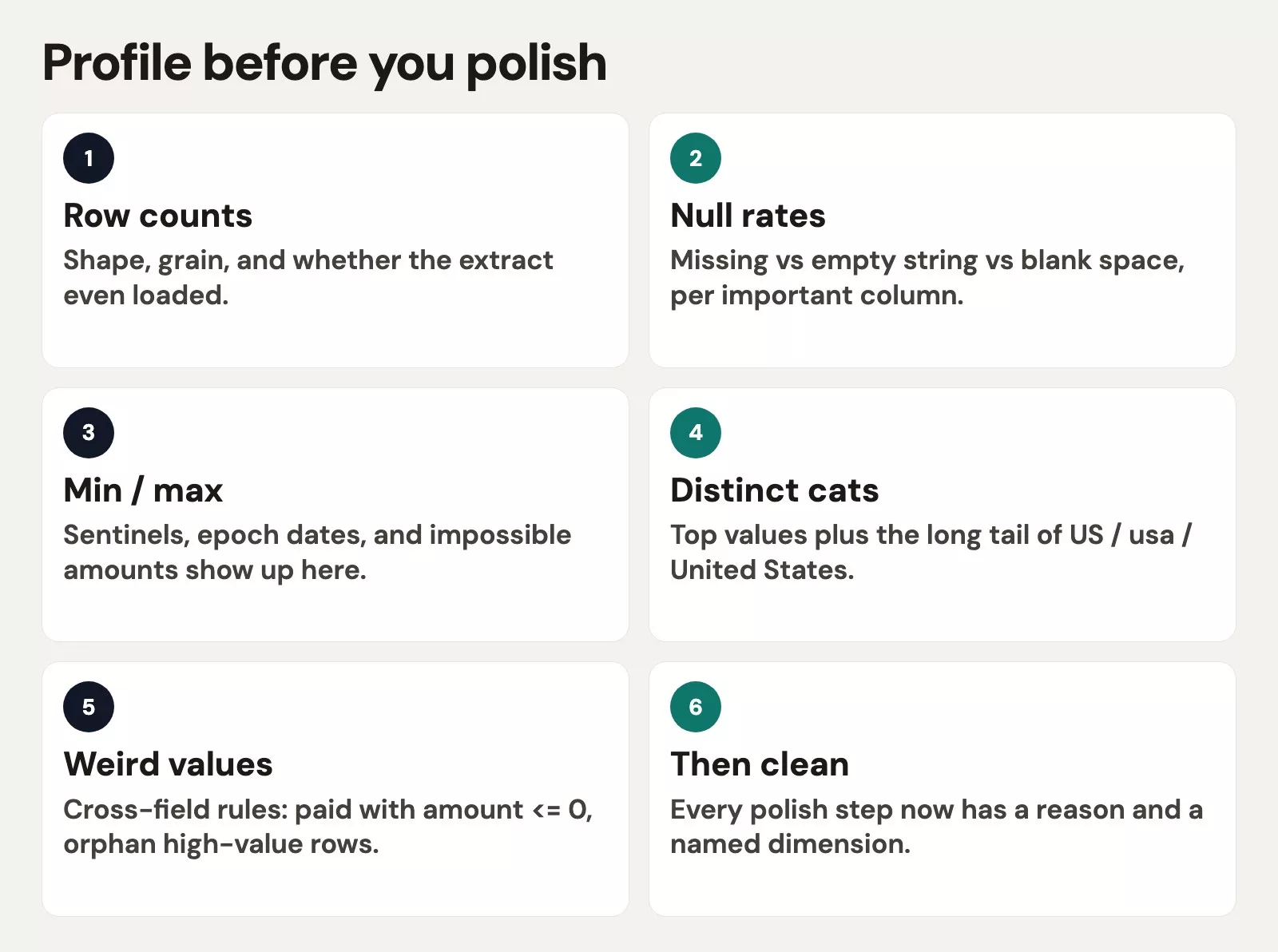
For any table that will feed a decision, capture the items in this list. A null is a cell with no value at all, and it is the most common gap you will find.
- Shape: row count, column list, primary key candidate
- Completeness: null or blank rate per important column
- Uniqueness: distinct counts vs rows for key columns
- Ranges: min, max, and a few quantiles for numbers and dates
- Categories: top values and long-tail oddballs for strings
- Freshness: max timestamp and lag vs “now” or report date
- Cross-field sanity: impossible combos (shipped with null ship date, negative prices on non-refund rows)
Write the findings in plain language so the person reading them can act. “3.2% of orders are missing a customer_id” is something a teammate can open a ticket for. “The data is messy” is only a mood, and nobody can fix a mood.
SQL: profile without changing anything
The examples assume a raw table named orders_raw. SQL dialects differ slightly (FILTER, IFF, and IFNULL are the usual differences), but the ideas carry over. If you are still building SQL skills, the SQL series covers the query pieces, and here we assemble them into a quality pass.
Shape, keys, and nulls
SELECT
  COUNT(*) AS row_count,
  COUNT(DISTINCT order_id) AS distinct_order_id,
  COUNT(*) - COUNT(DISTINCT order_id) AS duplicate_order_id_rows,
  COUNT(*) - COUNT(customer_id) AS null_customer_id,
  COUNT(*) - COUNT(order_ts) AS null_order_ts,
  ROUND(100.0 * (COUNT(*) - COUNT(customer_id)) / COUNT(*), 2) AS pct_null_customer_id
FROM orders_raw;
Example output:
If duplicate_order_id_rows is above zero, you already have a uniqueness problem. That comes before any talk of cleaning up categories, because every total built on those rows is counted more than once.
Numeric and date ranges
SELECT
  MIN(amount) AS min_amount,
  MAX(amount) AS max_amount,
  AVG(amount) AS avg_amount,
  MIN(order_ts) AS min_order_ts,
  MAX(order_ts) AS max_order_ts
FROM orders_raw;
Example output:
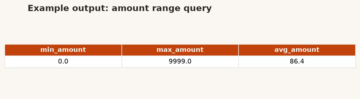
A maximum amount of 9,999,999.99 might be a sentinel, which is a fake placeholder number that a system stores when it has no real value. An order date in 1970 is usually a Unix epoch accident, meaning the computer counted from zero. A negative amount might be a refund, which is fine, or a sign error, which is not. Profiling raises the question, and your business rules answer it.
Category tails
SELECT
  status,
  COUNT(*) AS n,
  ROUND(100.0 * COUNT(*) / SUM(COUNT(*)) OVER (), 2) AS pct
FROM orders_raw
GROUP BY status
ORDER BY n DESC;
Example output:
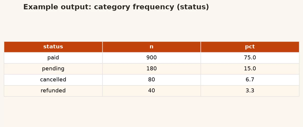
Run the same pattern for region, channel, currency, or any field people group by in dashboards. Look for near-duplicates such as US, usa, and United States. Also look for blank strings, and for catch-all groups like Other that quietly swallowed half the world.
Blank strings are not nulls
SELECT
  COUNT(*) FILTER (WHERE customer_email IS NULL) AS null_email,
  COUNT(*) FILTER (WHERE customer_email = '') AS empty_email,
  COUNT(*) FILTER (WHERE TRIM(customer_email) = '') AS blankish_email
FROM orders_raw;
Many tools treat an empty string as “present,” even though nothing is in it. Your completeness measure has to decide whether an empty string counts as missing. Profile both versions so the answer does not surprise you later.
Python: the same flashlight in pandas
When the data is a file, or you already work in notebooks, pandas is fast for a first pass. The official pages for DataFrame.describe, missing data, and value counts are worth bookmarking, and they are listed in Sources.
import pandas as pd

df = pd.read_csv("orders_raw.csv")

# Shape and dtypes
print(df.shape)
print(df.dtypes)

# Completeness: nulls and empty strings
nulls = df.isna().mean().sort_values(ascending=False)
empty_str = (df.select_dtypes("object").apply(lambda s: s.fillna("").str.strip().eq(""))).mean()
print(nulls.head(15))
print(empty_str.sort_values(ascending=False).head(15))

# Uniqueness on claimed keys
print(df["order_id"].duplicated().sum())
print(df.duplicated().sum())

# Ranges
print(df["amount"].describe())
print(df["order_ts"].min(), df["order_ts"].max())

# Categories: head and suspicious tail
print(df["status"].value_counts(dropna=False).head(20))
print(df["region"].value_counts(dropna=False).tail(20))
Example:
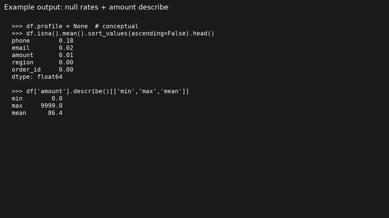
Many analysts keep a compact helper like this one around, so the same checks run the same way on every new file:
def quick_profile(df, key_cols=None, cat_cols=None):
    key_cols = key_cols or []
    cat_cols = cat_cols or df.select_dtypes("object").columns.tolist()
    out = {
        "rows": len(df),
        "cols": df.shape[1],
        "null_pct": df.isna().mean().to_dict(),
        "dup_full_rows": int(df.duplicated().sum()),
    }
    for k in key_cols:
        out[f"dup_{k}"] = int(df.duplicated(subset=[k]).sum())
        out[f"nunique_{k}"] = int(df[k].nunique(dropna=False))
    for c in cat_cols:
        out[f"top_{c}"] = df[c].value_counts(dropna=False).head(5).to_dict()
    return out

profile = quick_profile(df, key_cols=["order_id"], cat_cols=["status", "region"])
print(profile)
Paste the printout into the ticket. Future you will be glad the evidence is still there.
Worked example: orders that look fine until they don’t
Here is a miniature dataset. Suppose leadership wants the average order value by region for last week.
| order_id | customer_id | region | status | amount | order_ts |
|---|---|---|---|---|---|
| 5001 | 9 | US | paid | 40.00 | 2026-03-10 |
| 5002 | usa | paid | 55.00 | 2026-03-10 | |
| 5003 | 12 | EMEA | Paid | -15.00 | 2026-03-11 |
| 5004 | 12 | Europe | refunded | 15.00 | 2026-03-11 |
| 5005 | 18 | APAC | paid | 999999 | 2026-03-09 |
| 5001 | 9 | US | paid | 40.00 | 2026-03-10 |
| 5006 | 21 | pending | 22.00 | 1970-01-01 |
A blind cleaner might lowercase the statuses, fill the blank region with “Unknown,” drop the row with no customer_id, and delete the duplicate. A profiler slows down and writes down what each oddity probably means, as the next table shows.
| Finding | Likely dimension | Do not rush into… |
|---|---|---|
| Duplicate order_id 5001 | Uniqueness / load bug | Deleting without checking pipeline lineage |
| Null customer_id on 5002 | Completeness | Dropping the revenue row by reflex |
| US vs usa vs Europe vs EMEA | Consistency (representation) | Ad-hoc renames only in one chart |
| Paid vs paid | Consistency | Case-sensitive filters that undercount |
| amount -15 and 999999 | Accuracy / validity / business rules | Clipping outliers without refund logic |
| order_ts 1970-01-01 | Accuracy or defaulting bug | Including it in “last week” averages |
| Blank region | Completeness | Forcing a region to make the pivot pretty |
Now the cleaning plan has a spine, and you can follow it in order.
- Confirm what one row means: one paid order per
order_idfor average order value, with refunds kept separate. - Resolve the duplicate 5001 at the source, or with a written dedupe rule.
- Standardize the status spelling, and map regions through a mapping table (the later post on standardizing categories covers this).
- Define the amount rules: refunds as negative numbers or as separate rows, and cap or set aside 999999 only after the business confirms it.
- Exclude or repair the epoch dates with an explicit filter, not a silent deletion in a one-off notebook.
That is polish with a conscience. The numbers may still move, but this time you can explain why they moved.
Cross-field checks beat single-column vanity
Null rates for single columns are necessary but they are not enough on their own. Add a few rules that compare two columns and match how your business works. Each one finds a contradiction that no single column can show.
SELECT
  COUNT(*) FILTER (WHERE status = 'paid' AND amount <= 0) AS paid_nonpositive,
  COUNT(*) FILTER (WHERE status = 'refunded' AND amount > 0) AS refund_positive,
  COUNT(*) FILTER (WHERE order_ts::date < DATE '2000-01-01') AS ancient_dates,
  COUNT(*) FILTER (WHERE customer_id IS NULL AND amount > 100) AS high_value_orphan
FROM orders_raw;
The same rules in pandas look like this:
rules = {
    "paid_nonpositive": ((df["status"].str.lower() == "paid") & (df["amount"] <= 0)).sum(),
    "ancient_dates": (pd.to_datetime(df["order_ts"], errors="coerce") < "2000-01-01").sum(),
    "high_value_orphan": (df["customer_id"].isna() & (df["amount"] > 100)).sum(),
}
print(rules)
Each rule that returns a number above zero is a story to investigate, and a silent dropna would have hidden it.
From profile to ticket language
Translate your findings into the five quality dimensions from the earlier post, so engineers and stakeholders share one vocabulary. Each line below pairs a plain finding with the dimension it belongs to.
- “12% null
customer_idon paid orders” → completeness on a required field for customer-level metrics - “Max amount is a repeated 999999” → investigate accuracy / sentinel
- “Region has 47 variants for ~8 real markets” → consistency of categories
- “Max event time is 36 hours behind report time” → timeliness
- “1.8% duplicate primary keys” → uniqueness
This is also how you protect yourself. You are not “blocking on perfection.” You are documenting whether the data is fit for one named use, which is the same good-enough spirit as in the analytics foundations series.
Common mistakes
- Profiling only the columns you already like. The weird column is often the landmine.
- Using mean alone. Means hide spikes and sentinels. Keep min, max, and a high percentile.
- Trusting
describe()on messy types. If amount is stored as text, cast carefully after you see bad tokens. - Cleaning in the same cell as profiling. Separate “observe” and “transform” steps so you can undo.
- Skipping blank-string checks. Empty is not null in most SQL engines or pandas object columns.
- One-off profiles you never save. Stick the SQL or notebook snippet in the repo or ticket.
How to practice this week
- Pick one production table or CSV you ship from, and run the shape, null, range, and category queries above.
- Write five bullets: your biggest completeness risk, biggest uniqueness risk, weirdest category, weirdest range, and freshness lag.
- Add one cross-field rule that would embarrass you if leadership found the problem first.
- Refuse one quick-clean request until you paste a profile summary, and notice how the request changes.
- If SQL or pandas feel rusty, use the Learn page to jump into the path you need, then come back to the post on removing duplicates.
Quick recap
- Profile before you polish, and look before you change anything.
- Counts, nulls, ranges, categories, freshness, and cross-field rules are enough to start.
- SQL and Python both work, so use whichever tool sits closest to the data.
- Map each finding to a quality dimension so the fix matches the failure.
- The next post covers removing duplicates without destroying history, which is where you go when the uniqueness check fails.
Sources
- pandas documentation, “Working with missing data”: https://pandas.pydata.org/docs/user_guide/missing_data.html
- pandas API reference,
DataFrame.describe: https://pandas.pydata.org/docs/reference/api/pandas.DataFrame.describe.html - pandas API reference,
Series.value_counts: https://pandas.pydata.org/docs/reference/api/pandas.Series.value_counts.html - PostgreSQL aggregate documentation (COUNT, FILTER patterns): https://www.postgresql.org/docs/current/functions-aggregate.html
- IBM data quality dimensions (context for mapping profile metrics to dimensions): https://www.ibm.com/docs/en/ws-and-kc?topic=quality-data-dimensions
Keep going
Same lessons in your feed
Short diagrams, hooks, and weekly tutorials on Substack, Instagram, X, and Facebook.