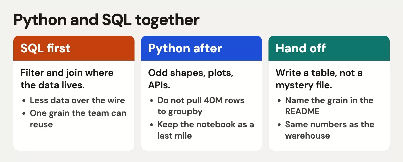
Python and SQL together

SQL people sometimes treat Python as a toy. Python people sometimes treat SQL as a dusty filing cabinet. Both are wrong in productive companies. The winning pattern is boring and powerful: let the database filter and aggregate close to the data, then use pandas for the awkward middle (reshapes, merges across exports, light models, handoff polish) that SQL makes painful.

This is Part 10 of Python for analytics, the closer for the core path. You can open a notebook without panic, shape DataFrames, merge carefully, clean nulls, run a small pipeline, and export like a professional. Now you put Python and SQL on the same team, including a healthy distrust of AI-generated code that “looks right.”

What you’ll learn

When SQL should win, when Python should win, and when either is fine
How to push filters and heavy aggregates into the database
A conceptual read_sql pattern with SQLite you can run locally
How to review AI-written SQL or pandas like a skeptical colleague
Where to go after this series (plotting and notebooks vs scripts as stretch goals)

Two tools, one question

Start with the decision, not the language. That is the habit from Analytics foundations. Once you know the grain and the filters, ask: where does the data live, how big is it, and who must maintain the logic?

If the warehouse already holds a curated table and your filter is “last 90 days for one brand,” SQL (or a metric layer on top of SQL) is usually faster, cheaper, and easier to govern. If you are combining a CRM CSV, a Google Ads export, and a manually adjusted finance sheet, pandas may be the least bad integration layer until engineering builds a real pipeline. The spreadsheets series already warned you about unofficial ledgers. Python does not make a bad multi-file process holy. It only makes it more automatable.

Job → preferred tool

Job	Prefer	Why
Filter 200M fact rows to 2M	SQL	Do not download a lake to your laptop
Standard revenue by month for finance	SQL / metric layer	One governed definition, many consumers
Join three messy vendor CSVs	Python	Flexible parsing, quick iteration
Exploratory reshape and “what if” columns	Python	Interactive, less DDL ceremony
Production daily aggregate tables	SQL (dbt/ELT)	Tests, lineage, schedules
One-off executive scenario model	Python or Sheets	Speed to answer; document assumptions
Row-level export for a partner	SQL extract or Python export	Whichever already has the clean table
ML feature sketch on a sample	Python	Libraries and iteration speed

Notice the pattern: big, shared, repetitive → SQL side. Awkward, multi-source, exploratory → Python side. Overlap exists. Arguments about purity waste time. Arguments about row counts and ownership save money.

Push filters to SQL

A classic anti-pattern is SELECT * FROM enormous_table into pandas, then filtering. Your laptop becomes a very expensive network cable. Push predicates and column lists down.

import sqlite3
import pandas as pd

# Demo database in memory (stand-in for warehouse / Postgres / BigQuery)
con = sqlite3.connect(":memory:")

# Seed a tiny "warehouse" table
seed = pd.DataFrame(
    {
        "order_id": [1, 2, 3, 4, 5, 6],
        "brand": ["A", "A", "B", "A", "B", "A"],
        "order_date": [
            "2024-05-01",
            "2024-06-02",
            "2024-06-03",
            "2024-06-10",
            "2024-04-01",
            "2024-06-20",
        ],
        "amount": [10.0, 15.0, 40.0, 12.0, 8.0, 22.0],
        "region": ["East", "East", "West", "West", "East", "East"],
    }
)
seed.to_sql("orders", con, index=False, if_exists="replace")

# Good: filter and select in SQL
sql = """
SELECT
  order_id,
  brand,
  order_date,
  amount,
  region
FROM orders
WHERE brand = ?
  AND order_date >= ?
"""

params = ("A", "2024-06-01")
orders_a = pd.read_sql_query(sql, con, params=params)
print(orders_a)
print("rows pulled", len(orders_a))

Example output:

Example output: SQL aggregate in pandas

Even in SQLite, the habit is right: parameters for values, explicit columns, filters in the query. On BigQuery, Snowflake, Redshift, or Postgres the same idea prevents scanning partitions you do not need. Your Python step should receive a decision-sized table when possible, not a souvenir copy of production.

Pull aggregates, then polish in Python

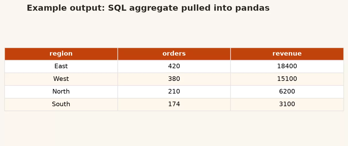
Example hybrid result table:

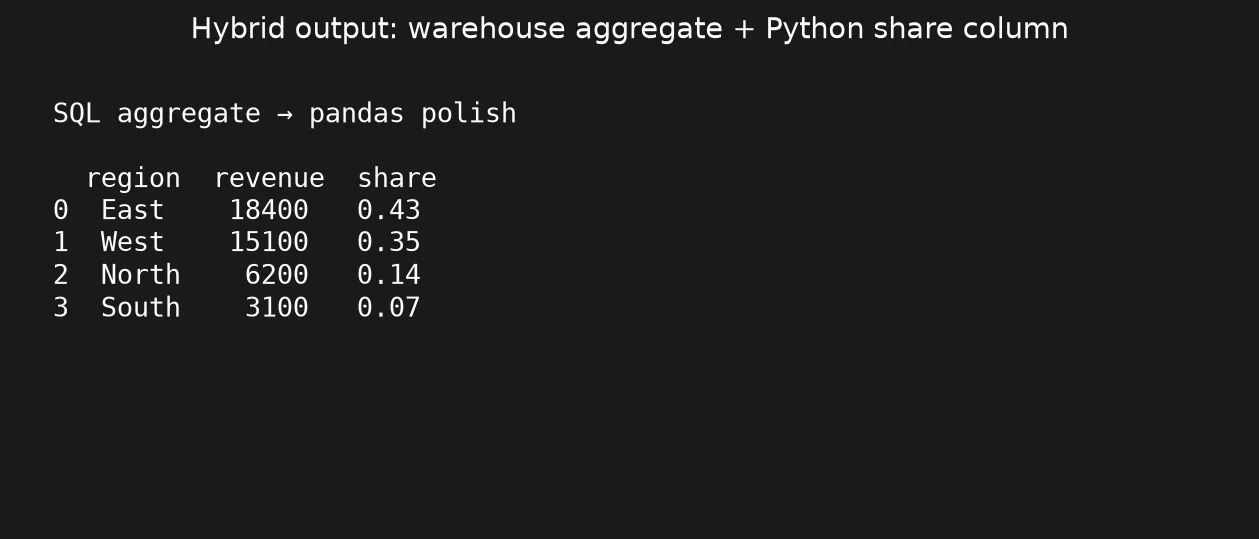
SQL aggregate polished with a share column in pandas.

Another strong hybrid: let SQL do the heavy groupby, then use pandas for presentation logic, secondary merges, or quick sensitivity scenarios.

agg_sql = """
SELECT
  region,
  COUNT(*) AS orders,
  SUM(amount) AS revenue
FROM orders
WHERE order_date >= ?
GROUP BY region
ORDER BY revenue DESC
"""

by_region = pd.read_sql_query(agg_sql, con, params=("2024-06-01",))

# Python polish: share of revenue, friendly labels, export-ready columns
by_region["revenue_share"] = by_region["revenue"] / by_region["revenue"].sum()
by_region["revenue_share_pct"] = (by_region["revenue_share"] * 100).round(1)
by_region["region_label"] = by_region["region"].fillna("Unknown")

print(by_region)

# Optional: merge a small mapping table that lives only as a CSV
region_owner = pd.DataFrame(
    {
        "region": ["East", "West"],
        "owner": ["Sam", "Alex"],
    }
)
handoff = pd.merge(by_region, region_owner, how="left", on="region", validate="one_to_one")
print(handoff)

Example:

SQL pull + share polish

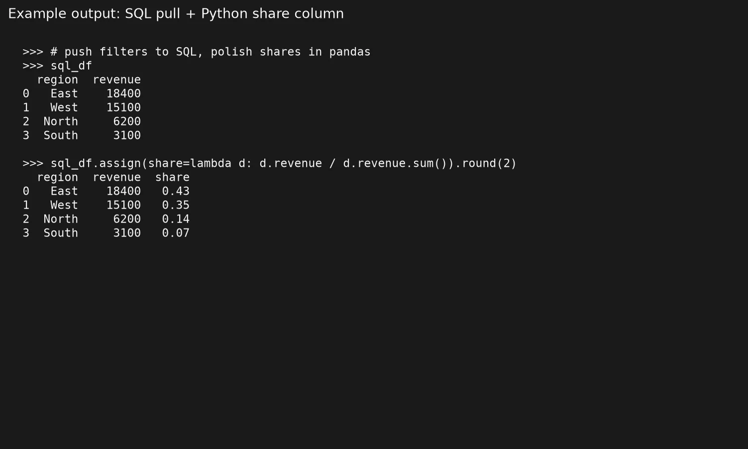
SQL computed the durable aggregate. Python attached a human mapping and percentage formatting for a slide or CSV handoff (Part 9). Neither tool needed to do everything.

A realistic split of responsibilities

SQL / warehouse: source of truth tables, access control, large scans, certified metrics, scheduled builds.
Python: multi-file glue, prototypes, custom scoring, complex string work, one-off investigations, export packaging.
Sheets: still fine for tiny models and stakeholder what-ifs, with the liability lessons from the spreadsheets series kept in mind.

When a Python prototype stabilizes and three teams depend on it weekly, that is a signal to promote logic into tested SQL models or a proper job, not a signal to add more notebook cells forever.

AI-generated code: useful draft, untrusted finish

Models can draft SQL and pandas quickly. They also invent join keys, forget grain, and filter the wrong date column with total confidence. Treat generated code like a junior teammate’s first pass: helpful, not authoritative.

Review checklist before you run anything on real data:

Grain: What does one output row mean? Say it out loud.
Keys: Are join keys unique on the side you assume? Would validate= pass?
Filters: Time zone, inclusive vs exclusive end dates, deleted rows, test accounts.
Null policy: Does WHERE status = 'active' drop null statuses you still need?
Fanout: Could a merge multiply revenue?
Scope: Does the query scan far more history than the question needs?
Secrets: Never paste production credentials into a chat tool. Use env vars and approved clients.

If you use AI to draft SQL, compare it to patterns you learned in the SQL series: explicit columns, intentional joins, and checks on row counts. If you use AI to draft pandas, compare it to Parts 6 through 9 of this series: merge validation, dtype coercion with reports, and export metadata. For broader learning paths and related tutorials, start at the Learn hub.

Worked micro workflow

End-to-end sketch you can adapt:

Write the business question and grain in one sentence each.
Draft SQL that returns the smallest sufficient table (filters + columns + maybe aggregates).
Pull with read_sql (or your warehouse client) into pandas.
Run Part 7 cleaning only for what SQL did not already enforce.
Merge any local reference files with validate and row-count prints (Part 6).
Summarize or scenario-model in Python.
Export with metadata (Part 9). Store the SQL text next to the pipeline.

def pull_brand_orders(con, brand: str, start_date: str) -> pd.DataFrame:
    sql = """
    SELECT order_id, brand, order_date, amount, region
    FROM orders
    WHERE brand = ?
      AND order_date >= ?
    """
    df = pd.read_sql_query(sql, con, params=(brand, start_date))
    df["order_date"] = pd.to_datetime(df["order_date"], errors="coerce")
    df["amount"] = pd.to_numeric(df["amount"], errors="coerce")
    print(f"pulled brand={brand} rows={len(df)} null_amounts={df['amount'].isna().sum()}")
    return df

def region_share(df: pd.DataFrame) -> pd.DataFrame:
    g = (
        df.groupby("region", dropna=False, as_index=False)
        .agg(orders=("order_id", "count"), revenue=("amount", "sum"))
    )
    g["revenue_share"] = g["revenue"] / g["revenue"].sum()
    return g.sort_values("revenue", ascending=False)

sample = pull_brand_orders(con, "A", "2024-06-01")
print(region_share(sample))
con.close()

Small functions, SQL at the edge, pandas in the middle, prints for trust. That is the adult hybrid.

Governance without bureaucracy

Hybrid workflows fail when nobody owns the metric definition. If Finance certifies revenue in the warehouse, your pandas notebook should consume that certified grain, not reinvent a cousin metric with a friendlier filter. If no certified table exists, say so in the handoff: “prototype definition, not official revenue.” Clarity beats territorial arguments.

A lightweight rule that works in many teams: SQL models hold definitions that multiple people will reuse next month. Python holds investigations and glue that may never run again. When a Python path runs every week and three stakeholders depend on it, schedule a promotion conversation. Promotion might mean dbt, a scheduled SQL job, or simply a reviewed script with tests. The point is intentionality, not tool fashion.

Document the split in the same place you document the pipeline: which filters live in SQL, which enrichments live in Python, and which number is allowed on an external slide. That one paragraph prevents duplicate logic better than a long architecture debate.

Common mistakes

Downloading everything “just in case.” Case closed: your RAM and your bill both suffer.
Reimplementing certified metrics in pandas with slightly different filters, then arguing with Finance.
Putting business logic only in a BI calculated field and only in a notebook, twice, differently.
Trusting AI joins without checking multiplicity.
Leaving SQL as a string with no parameters while concatenating user input (injection risk in apps; mess risk in analytics).
Stopping at a chart with no saved query or pipeline, so the next person starts from zero.

Practice

Pick one weekly question you currently answer with a giant sheet export. Rewrite it as: (1) a SQL query that returns a tight extract, (2) a pandas step that finishes the story, (3) a CSV plus meta note. Time yourself. Compare correctness to the old process. The goal is not fewer tools. The goal is fewer surprises.

Closing the core series (and what is next)

If you followed Python for analytics from Part 1 through Part 10, you now have a practical spine:

Choose Python when it earns its keep (Part 1)
Set up without tears (Part 2)
Treat DataFrames as tables (Part 3)
Select, filter, sort (Part 4)
Aggregate with groupby (Part 5)
Merge with grain discipline (Part 6)
Handle missing data and dtypes (Part 7)
Pipeline for reproducibility (Part 8)
Export and hand off (Part 9)
Partner with SQL and review generated code (Part 10)

Stretch goals when you are ready: plotting for analysis (one chart stack, used for exploration and explanation), and notebooks versus scripts for sharing with teammates. Those topics deepen the craft. They are not required to do useful work Monday. Many analysts deliver real value with clean tables, honest joins, and clear handoffs long before they perfect a visualization library.

Keep SQL sharp via the SQL series. Keep sheet hygiene via From spreadsheets to real data. Browse everything on the Learn hub. And when a number matters, still ask what problem you are solving before you open either a query window or a notebook.

Quick recap

SQL wins on large, shared, governed transforms; Python wins on messy glue and exploration.
Push filters and heavy aggregates down; pull decision-sized tables up.
read_sql plus pandas polish is a standard hybrid, not a compromise.
AI drafts need grain, key, filter, and fanout review before trust.
You finished the core Python path; plotting and packaging styles are optional next climbs.

Sources

pandas read_sql_query: https://pandas.pydata.org/docs/reference/api/pandas.read_sql_query.html
Python sqlite3 module: https://docs.python.org/3/library/sqlite3.html
pandas comparison with SQL: https://pandas.pydata.org/docs/getting_started/comparison/comparison_with_sql.html
SQLite documentation: https://www.sqlite.org/docs.html
Analytics Made Simple, SQL series: https://analyticsmadesimple.com/series/sql/
Analytics Made Simple, Learn hub: https://analyticsmadesimple.com/learn/