Sampling and bias for analysts

Someone drops a chart in Slack with a confident caption: “Customers love the new checkout.” The conversion rate jumped. The sample is last week’s mobile sessions in the US. Finance is already writing the win into the forecast. Then support asks a quiet question: did we measure all customers, or only the ones who still made it far enough to load the new page?

That is sampling and bias in one meeting. You rarely get a clean census of reality. You get a slice. The slice can still be useful. It becomes dangerous when you pretend the slice is the whole world, or when the missing people are exactly the people who would have changed the story.

This is Part 1 of Statistics for analysts, a short series for people who ship dashboards, write SQL, and get asked whether a number is “significant” before anyone has defined the population. We start with sampling and bias because every later topic (group comparisons, confidence intervals, A/B tests) inherits the sample you chose, or the sample your product funneled to you.

What you’ll learn

How to name population, sample, sampling frame, and unit of analysis without sounding like a textbook
The bias types that show up most often in analytics work (selection, survivor, response, measurement, and convenience)
Why “random” in product analytics is rarely the same as random in a survey textbook
A worked example that turns a misleading NPS slice into a defensible sampling write-up
A practical checklist you can put above any chart before you defend it in a meeting

Population, sample, and the story you are allowed to tell

Start with four labels. Write them once for every analysis that will leave your laptop.

Population: the full set of units you care about for the decision (all active subscribers in Q3, all warehouse SKUs that ship weekly, all support tickets opened last month).
Sampling frame: the list or system you can actually reach (users with email, events in the warehouse, accounts that still exist after a migration).
Sample: the units you actually measure (the 2,400 survey responses, the 10% of sessions with client logging on, last Tuesday’s cohort).
Unit of analysis: what one row means (user, account, session, order, day). Mixing units is a classic way to invent growth.

If population and frame differ, say so. If frame and sample differ, say so. Most “the data shows” arguments fail because someone silently swapped those layers. The decision may still be fine. The language should match the reach of the evidence.

Rule of thumb: Your conclusion may only be as wide as the population you can honestly name. Everything else is speculation with a chart attached.

This discipline pairs with metric definition work in the metrics series: you cannot sample “engagement” until you define the event. Sampling sits on top of definitions. Bad definitions make beautiful samples that answer the wrong question.

How samples form in real analytics work

Textbooks love simple random samples. Product and business data usually give you one of these instead.

Census of a system (still not “everyone”)

You pull every row from a table. That feels complete. It is complete only for that system’s history of what it recorded. Deleted users, failed events, blocked trackers, and regions where the feature never shipped are still missing. A warehouse full table is a census of the frame, not always a census of the population.

Convenience and operational samples

Last week’s logs. The accounts your CSM team knows. The tickets tagged “billing.” These samples are easy and often useful for operational firefighting. They are weak for claims about “all customers” unless you can argue the convenience path is unrelated to the outcome you care about. It usually is related.

Probability samples (surveys, panels, some research pulls)

Here each unit has a known chance of selection. You can weight, estimate error, and talk more carefully about generalization. Most day-to-day product analytics is not this. When you do run a survey, document the response rate and who never opened the email. Nonresponse is its own sample filter.

Experiment assignment (designed sample)

A/B tests create treatment and control samples on purpose. Random assignment helps causal claims inside the experiment population. It does not magically fix a narrow eligibility filter. If only power users enter the experiment, your result is about power users. Parts 3 and 4 of this series and the experimentation culture series go deeper. Sampling starts the honesty chain.

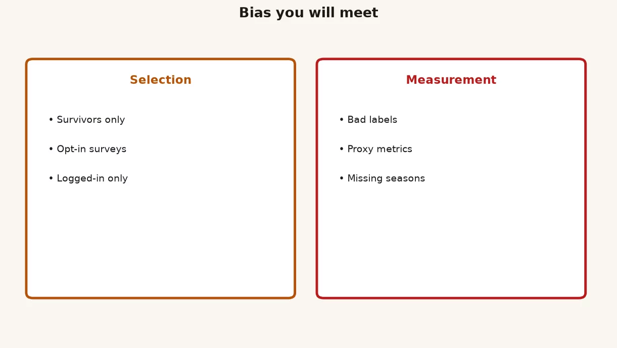
Diagram of population, sampling frame, and sample with arrows showing who is excluded at each layer

Bias types analysts actually meet

Bias here means a systematic tilt, not a mean comment in a spreadsheet. Random noise averages out with more data. Bias does not. More biased data can make you more confident in the wrong story.

Selection bias

The process that gets units into your sample correlates with the outcome. Example: you study feature adoption using only users who opened the product at least five times. Heavy users look like they love everything. Light users who bounced never enter the table. Your adoption rate is conditioned on survival into the product, not on the full signup cohort.

Survivor bias

You only see the units that lasted. Classic business version: average revenue of current customers ignores churned accounts. Classic career version: studying “what successful startups did” without the failed ones that did the same things. In analytics, retention tables that start at “users still active in month 6” hide the early exits that define the product risk.

Response and self-selection bias

Surveys, reviews, and optional feedback forms over-index on people with strong feelings or free time. A 12% response rate is not a small random sample. It is a volunteer army. If you publish “customers rate us 9.1,” add who was invited, who answered, and how answers differ by plan tier if you can measure that.

Measurement bias

The instrument tilts the answer. Client-side events miss users with blockers. Server-side counts may miss client-only frustration. A 1-5 CSAT scale with “5” labeled “ecstatic” and no “4.5” option still shapes scores. Timezone cuts, currency conversions, and late-arriving events all measure something adjacent to the truth you named.

Confounding dressed up as sampling

You compare markets, but one market got a promo and a different sales motion. The “sample of Germany vs France” is also a sample of different treatments. Part 2 covers comparing groups. For now, notice that your sample description should list co-traveling conditions, not only geography labels.

Bias flavor	Monday morning tell	What to write in the chart note
Selection	“We only looked at users who…”	Eligibility rule and who failed it
Survivor	Averages on current base only	Include churned / inactive definition
Response	Optional survey or review data	Invite count, response rate, channel
Measurement	Tracker gaps, late events	Known coverage holes by platform
Convenience	“I used the export I already had”	Why this slice, and what is out of scope

Coverage, missingness, and “null is a person”

Missing data is not only a data quality ticket. Missingness is often a sampling story. If mobile web has higher null rates on device fields, any cut by device type is also a cut by instrumentation quality. If new markets have incomplete CRM fields, “complete profiles convert better” may mean “complete profiles are older markets with better ops,” not that form completeness causes conversion.

When you drop nulls without a write-up, you silently redefine the sample. Prefer reporting rates both ways when the drop is large: including unknowns as a category, and excluding them with a clear exclusion rate. The data quality series pairs well here: quality issues become statistical issues the moment you summarize.

Worked example: the NPS slide that flattered the product

Imagine a B2B SaaS product. Product wants a headline NPS for the board. Ops pulls every response from the in-app survey for the last 90 days. Score: +42. Caption: “Customers are promoters.” You are the analyst who has to decide whether that sentence is allowed.

You reconstruct the path:

Population claimed: all customers.
Frame: users who logged into the app (survey is in-product only).
Trigger: shown after three successful workflows in a week (happy path bias).
Response: 18% of those who saw the prompt answered.
Unit: user-level scores, but board decisions are account-level (power users in large accounts answer more).

You rebuild a transparent version of the table. Numbers below are a teaching toy, labeled as such, not a real company result.

Slice	Invited or eligible	Responded	NPS
All active accounts (CRM)	12,400 accounts	n/a	unknown
Users who logged in (90d)	41,200 users	n/a	unknown
Saw in-app prompt	9,800 users	1,764	+42
Enterprise plan responders	n/a	610	+51
Free or trial responders	n/a	220	+9
Accounts with a churn risk flag	n/a	95	-8

Honest board language becomes: “Among users who completed three workflows and chose to answer an in-app survey (about 4% of logged-in users), NPS was +42, higher on enterprise seats. We do not yet have a probability sample of all accounts, and churn-risk accounts who answered score poorly.” That sentence is longer. It is also true. Truth is a feature.

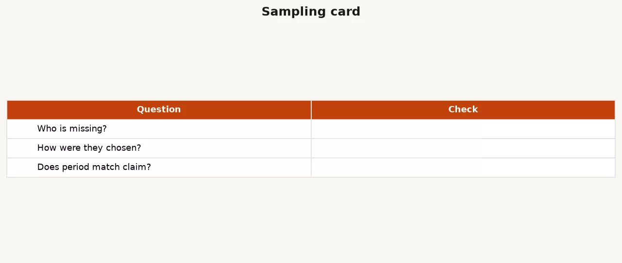
Result card comparing claimed population all customers versus actual sample of in-app survey responders with NPS plus 42

A short SQL pattern for documenting the funnel into the sample

You do not need fancy stats packages to start. Count the funnel that creates the sample and keep those counts next to the metric.

WITH base AS (
  SELECT user_id, account_id, plan_tier
  FROM users
  WHERE last_login_at >= CURRENT_DATE - INTERVAL '90' DAY
),
prompted AS (
  SELECT DISTINCT user_id
  FROM survey_impressions
  WHERE survey_id = 'nps_inapp_v3'
    AND impressed_at >= CURRENT_DATE - INTERVAL '90' DAY
),
answered AS (
  SELECT user_id, nps_score, submitted_at
  FROM survey_responses
  WHERE survey_id = 'nps_inapp_v3'
    AND submitted_at >= CURRENT_DATE - INTERVAL '90' DAY
)
SELECT
  (SELECT COUNT(*) FROM base) AS logged_in_users,
  (SELECT COUNT(*) FROM prompted) AS saw_prompt,
  (SELECT COUNT(*) FROM answered) AS responded,
  ROUND(100.0 * (SELECT COUNT(*) FROM answered)
    / NULLIF((SELECT COUNT(*) FROM prompted), 0), 1) AS response_rate_pct
;

Put those four numbers in the slide footer. People argue less with footers that contain arithmetic.

How much sample is “enough”?

Enough for what? A directional product gut check can use a small, biased sample if everyone agrees the goal is “what are angry power users saying,” not “what does the market believe.” A pricing decision that moves millions needs a sample design that matches the stakes. Sample size calculators matter later for experiments (Part 4). Before size, fix composition. A huge biased sample is still biased. A modest representative sample can beat a giant convenience dump.

Practical analyst move: state the decision’s cost of being wrong, then state the sample’s reach. If those two feel mismatched, stop decorating the chart and redesign the measurement plan.

Writing sample notes people will actually read

Keep a four-line block under any external-facing number:

Who is in: eligibility in one sentence.
Who is out: the largest excluded groups.
When: date range and any odd seasons (launches, outages, holidays).
How measured: event source, survey channel, or definition link.

If you cannot fill those lines, you are not ready to defend the number. Related hygiene lives in data stewardship and in clear metric contracts. Sampling notes are stewardship for statistical claims.

Common mistakes

Calling a warehouse extract “unbiased” because it was large. Size is not fairness.
Dropping nulls without reporting the drop rate. You redefined the sample in silence.
Mixing units (sessions vs users vs accounts) mid-story so growth appears from double counting.
Generalizing from log-in users to all customers when many customers are offline, multi-seat, or API-only.
Using early adopter cohorts as the voice of the mass market after a beta that required invitation.
Treating experiment traffic as product-wide truth when eligibility was narrow.
Publishing survey scores without response rate as if silence were random.

How to practice

Pick one dashboard KPI you show weekly. Write population, frame, sample, and unit in four lines.
Estimate (even roughly) who is excluded. Name the biggest excluded group out loud to a teammate.
Add a footer with coverage or response rates for any survey-like metric.
Find one place where null-dropping changes a rate by more than a few points. Document both versions.
Optional: rebuild a “who enters the metric” funnel in SQL for a single important score.

Next in this series: comparing groups without fooling yourself (baselines, mix shifts, and apples-to-apples cuts). For a broader map of skills, use the Learn hub. When AI helps you draft SQL for these funnels, still verify filters the way you would in how to check AI-written SQL.

Quick recap

Every analysis has a population, a frame, a sample, and a unit. Name them.
Bias is systematic tilt. More data does not automatically fix it.
Product data is often a convenience or system census sample, not a textbook random sample.
Missingness and eligibility rules are sampling decisions, not only engineering bugs.
Honest footers (who is in, who is out, when, how measured) prevent overclaiming.
Match sample reach to decision stakes before you polish the chart.

Sources

Lohr, Sharon L. Sampling: Design and Analysis (concepts of frames, bias, and design). Overview via CRC / Chapman & Hall listings and course syllabi; start with any solid sampling text your library holds. Companion overview: U.S. Census Bureau sampling methodology notes as a public example of frame thinking: https://www.census.gov/programs-surveys/sipp/methodology/sampling.html
Pew Research Center. “Methods 101” and survey methodology explainers (nonresponse and representativeness in plain language). https://www.pewresearch.org/our-methods/
OpenIntro Statistics (free). Sampling and bias chapters for intuition without heavy formalism. https://www.openintro.org/book/os/
Google Optimize / GA4 documentation on data-driven attribution and data thresholds is product-specific, but Google’s analytics help on data collection limits is a useful reminder that “all hits” still have coverage rules: https://support.google.com/analytics/answer/9304153
NIH / National Library of Medicine primers on selection bias in observational research (transferable language for product analytics). Example overview: https://www.ncbi.nlm.nih.gov/books/NBK436351/