SQL Tutorial 10: Advanced SQL Techniques

Some questions refuse to fit in a single flat SELECT. You need step one, then step two, then a ranking inside each region. Nested subqueries can do it, but your future self will need a decoder ring. Common table expressions (CTEs) name those steps. Window functions compute rankings and running totals while keeping detail rows. Recursion handles “walk the tree” problems when you are ready. Together they are how intermediate SQL starts to feel like programming with tables.

This is Part 10 of the SQL series. Part 7 nested queries. Part 9 named views. Now you name temporary result sets inside one statement and compute across related rows without collapsing them with GROUP BY. Follow the path on the SQL series page and the wider map on Learn.

What you will learn

How WITH … AS builds readable multi-step queries (CTEs)
When a CTE beats a nested subquery for humans
Window functions: ROW_NUMBER, SUM() OVER, partitions and order
How windows differ from GROUP BY (detail rows stay)
Recursive CTEs at a conceptual level with a small example
Worked patterns on the customers and orders toy data

Map of the advanced toolkit

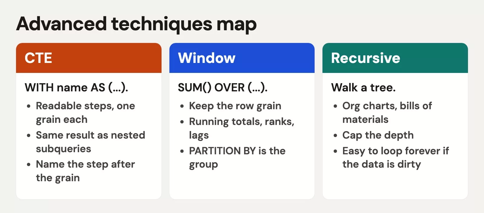
You do not need every tool every day. CTEs improve almost any multi-step analysis. Windows unlock rankings, percentiles, and period comparisons without losing row grain. Recursion is rarer in commercial analytics but essential for org charts, category trees, and bill-of-materials style data when that is your domain.

CTEs: name the steps in one query

A common table expression starts with WITH, defines one or more named subqueries, then runs a final SELECT (or other statement, depending on engine) that uses those names. Think of sticky notes on a whiteboard: “paid_orders,” “spend_by_customer,” “final_list.”

WITH paid_orders AS (
  SELECT
    order_id,
    customer_id,
    order_date,
    amount
  FROM orders
  WHERE status = 'paid'
),
spend_by_customer AS (
  SELECT
    customer_id,
    SUM(amount) AS total_spend,
    COUNT(*) AS order_count
  FROM paid_orders
  GROUP BY customer_id
)
SELECT
  c.name,
  c.region,
  s.total_spend,
  s.order_count
FROM spend_by_customer AS s
INNER JOIN customers AS c
  ON c.customer_id = s.customer_id
WHERE s.total_spend >= 150
ORDER BY s.total_spend DESC;

Compare that to the nested derived-table version from Part 7. Same idea, less nesting. Reviewers can discuss each CTE by name. You can comment each block. When AI tools generate SQL, asking them to use CTEs often produces something humans can audit faster.

CTEs are not automatically faster than subqueries. Some engines inline them; some materialize them. Write CTEs for clarity first. If a plan shows a problem, measure and adjust (Part 12). Clarity still wins for weekly metrics that must stay correct.

Think of CTEs as the outline view of your analysis. Each name should be a noun phrase a teammate understands: paid_orders, spend_by_customer, region_ranks. Avoid names like t1 and temp unless you are truly mid-refactor. Good names reduce the need for long comments. Bad names force every reader to re-derive your intent from the SELECT list alone.

Another practical win: you can comment each CTE with the grain it produces. “One row per paid order.” “One row per customer.” “One row per region rank slot.” Those comments prevent the classic mistake of joining two customer-grain CTEs and accidentally treating the result as order-grain. The database will not save you from a logical grain error. Naming and comments will.

Multiple CTEs and reuse

You can reference earlier CTEs from later ones, as above. That reuse is exactly why the East above-average story from Part 7 becomes saner: define per_customer once, compute the average from it, then filter against that average without pasting the aggregate twice.

WITH per_customer AS (
  SELECT
    customer_id,
    SUM(amount) AS total_spend
  FROM orders
  WHERE status = 'paid'
  GROUP BY customer_id
),
avg_spend AS (
  SELECT AVG(total_spend) AS threshold
  FROM per_customer
)
SELECT
  c.customer_id,
  c.name,
  p.total_spend,
  a.threshold
FROM per_customer AS p
INNER JOIN customers AS c
  ON c.customer_id = p.customer_id
CROSS JOIN avg_spend AS a
WHERE c.region = 'East'
  AND p.total_spend > a.threshold
ORDER BY p.total_spend DESC;

CROSS JOIN avg_spend attaches the single threshold row to every candidate. Some people prefer a scalar subquery for the threshold. Either is fine when the CTE keeps the definition of spend consistent.

Window functions: aggregates that keep the rows

GROUP BY collapses many rows into one summary row per group. A window function computes a value from a related set of rows (the window) but returns a result on each input row. That is how you rank orders inside a customer, compute a running total, or compare each day to the prior day without losing detail.

Core pieces:

Function: ROW_NUMBER(), RANK(), SUM(), AVG(), LAG(), and friends
OVER (…): defines the window
PARTITION BY: restart the calculation per group (like a GROUP BY that does not collapse)
ORDER BY inside OVER: defines sequence for ranking and running calculations
Frame clause (advanced): which rows relative to the current row participate (defaults matter)

ROW_NUMBER: label rows in order

Business ask: for each customer, show their most recent paid order only.

WITH ranked AS (
  SELECT
    o.order_id,
    o.customer_id,
    o.order_date,
    o.amount,
    ROW_NUMBER() OVER (
      PARTITION BY o.customer_id
      ORDER BY o.order_date DESC, o.order_id DESC
    ) AS rn
  FROM orders AS o
  WHERE o.status = 'paid'
)
SELECT
  r.order_id,
  c.name,
  r.order_date,
  r.amount
FROM ranked AS r
INNER JOIN customers AS c
  ON c.customer_id = r.customer_id
WHERE r.rn = 1
ORDER BY r.order_date DESC;

ROW_NUMBER assigns 1, 2, 3 within each customer ordered by date. Filtering rn = 1 keeps the latest. The extra order key order_id breaks ties so the result is stable. RANK and DENSE_RANK handle ties differently if you need competition-style ranking later.

Example output:

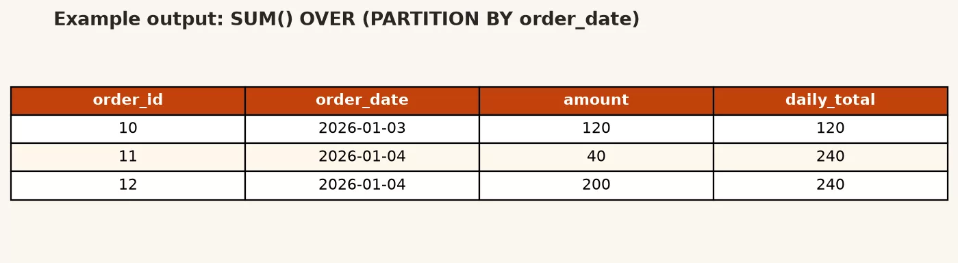
SUM OVER: running and group totals beside detail

Business ask: list each paid order with the customer’s lifetime paid spend on the same row (detail plus context).

SELECT
  o.order_id,
  o.customer_id,
  o.order_date,
  o.amount,
  SUM(o.amount) OVER (
    PARTITION BY o.customer_id
  ) AS customer_paid_total,
  SUM(o.amount) OVER (
    PARTITION BY o.customer_id
    ORDER BY o.order_date, o.order_id
  ) AS running_paid_total
FROM orders AS o
WHERE o.status = 'paid'
ORDER BY o.customer_id, o.order_date, o.order_id;

Without ORDER BY inside OVER, SUM over a partition is the full group total on every row. With ORDER BY, many engines default to a running total from the start of the partition through the current row. Always check your dialect’s default frame if numbers look “too cumulative” or “not cumulative enough.” The teaching point is solid: windows let you hang aggregate context on detail rows.

Example output:

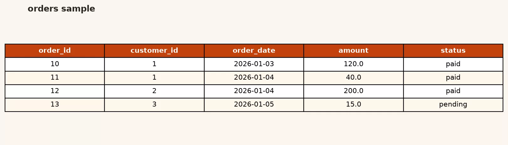
GROUP BY versus windows: choose by output grain

Need	Prefer	Output grain
One summary row per region	GROUP BY	Region
Each order plus regional rank	Window	Order (detail)
Latest order per customer	Window + filter, or distinct-on style dialect feature	One order per customer
Dashboard KPI cards only	GROUP BY (or metric layer)	KPI

If you GROUP BY too early, you lose the rows you wanted to rank. If you window when you only needed a chart of five regional totals, you ship unnecessary detail. Match the tool to the grain the decision needs. That is the same grain discipline you practiced with joins.

Recursive CTEs: conceptual walk-through

A recursive CTE references itself to walk hierarchical data. Support and syntax vary by engine, but the shape is usually: an anchor member (starting rows) UNION ALL a recursive member (how to find the next level), with a termination condition when no new rows appear.

Tiny conceptual example: numbers from 1 to 5 (not business data, but perfect for seeing the loop):

WITH RECURSIVE n AS (
  SELECT 1 AS value
  UNION ALL
  SELECT value + 1
  FROM n
  WHERE value < 5
)
SELECT value
FROM n
ORDER BY value;

Anchor produces 1. Recursive step adds 1 until the filter stops the growth. Real hierarchies replace numbers with parent/child keys: employee reports-to manager, product category parent, ticket blocked-by ticket. Safety notes: always have a stop condition, watch for cycles in dirty data, and cap depth if your engine allows. Do not recurse over unbounded graphs in production without guardrails.

If your workplace never models trees in SQL, you can skim recursion and still be highly effective with CTEs and windows. If you do model trees, practice on a small org chart table before touching production hierarchies.

A realistic mini hierarchy for practice is product categories: Electronics → Phones → Accessories, with each row pointing at a parent category id. The recursive walk collects a category and all descendants so a report can include “Phones and everything under Phones.” The same pattern shows up in manager chains and ticket dependency graphs. Dirty data with cycles (A parent of B, B parent of A) will loop until the engine stops you. That is why cycle detection or depth caps belong in production recursive SQL, not only in textbooks.

Worked story: regional leaderboard of customers

Ask: within each region, rank customers by paid spend and keep the top 2.

WITH paid_spend AS (
  SELECT
    c.customer_id,
    c.name,
    c.region,
    SUM(o.amount) AS total_spend
  FROM customers AS c
  INNER JOIN orders AS o
    ON o.customer_id = c.customer_id
  WHERE o.status = 'paid'
  GROUP BY c.customer_id, c.name, c.region
),
ranked AS (
  SELECT
    customer_id,
    name,
    region,
    total_spend,
    ROW_NUMBER() OVER (
      PARTITION BY region
      ORDER BY total_spend DESC, customer_id
    ) AS region_rank
  FROM paid_spend
)
SELECT
  region,
  region_rank,
  name,
  total_spend
FROM ranked
WHERE region_rank <= 2
ORDER BY region, region_rank;

Step one aggregates to customer grain. Step two ranks inside region. Step three filters. Each CTE is testable: you can temporarily SELECT from paid_spend alone while debugging. That is professional SQL, not clever one-liners.

LAG, LEAD, and a calm note on frames

Once ROW_NUMBER and SUM() OVER feel natural, two more window helpers show up constantly in business timelines. LAG looks at a previous row in the window order. LEAD looks ahead. Classic use: compare each day’s revenue to the prior day without a self-join.

WITH daily AS (
  SELECT
    order_date,
    SUM(amount) AS paid_revenue
  FROM orders
  WHERE status = 'paid'
  GROUP BY order_date
)
SELECT
  order_date,
  paid_revenue,
  LAG(paid_revenue) OVER (ORDER BY order_date) AS prev_day_revenue,
  paid_revenue
    - LAG(paid_revenue) OVER (ORDER BY order_date) AS day_over_day_change
FROM daily
ORDER BY order_date;

The first day has no previous value, so LAG returns null. That is expected. Do not “fix” it with zero unless zero is a true business claim about a day with no history.

Frames control which rows inside a partition participate for ordered windows. Defaults differ slightly by function and engine, which is why running totals sometimes surprise people. If numbers look cumulative when you wanted the whole partition, or the reverse, read your engine’s docs for ROWS BETWEEN and RANGE BETWEEN. You do not need every frame option on day one. You need to know frames exist so you do not invent superstitions when a total looks “off by one group.”

Workplace guidance: use windows to keep detail grain when stakeholders still want line-level tables with context columns. Use GROUP BY when they only want the summary chart. Use CTEs to keep both readable. If a single statement grows past a screen, split CTEs more aggressively rather than nesting windows inside subqueries inside joins until the plot is lost.

Common mistakes

Using ROW_NUMBER without a deterministic ORDER BY, then wondering why “top” flips between runs.
Confusing RANK and ROW_NUMBER on ties (two people share rank 1 with RANK; ROW_NUMBER never ties).
Grouping away the rows you needed to window. Sequence: filter, window, then aggregate if needed.
Assuming CTEs always materialize or never materialize. Check plans when performance matters.
Recursive queries without cycle protection on real hierarchies that contain bad parent pointers.
Copying window SQL from another dialect without checking frame defaults and function support.

Rule of thumb: If a nested subquery needs a diagram, rewrite it as CTEs. If a GROUP BY destroys rows you still need on the page, reach for a window.

How to practice

Rewrite your favorite Part 7 nested query as a two or three CTE pipeline.
Compute each customer’s paid order rank by amount and filter to their top order.
Add a running total of paid amount ordered by date for one customer_id.
Run the recursive numbers example, then invent a tiny parent/child category table and walk two levels.
Export a window query result to CSV and chart it in Python if you like visual checks from the Python series.

Quality angle: rankings amplify dirty duplicates. If one person has two customer_ids, they appear twice on the leaderboard. Window functions do not clean master data. Pair with data quality habits when stakes are high.

Quick recap

CTEs name intermediate steps inside one statement for readable multi-step logic.
Window functions compute across related rows while keeping detail grain.
ROW_NUMBER ranks; SUM() OVER can show group totals or running totals.
Recursive CTEs walk hierarchies with anchor plus recursive members and stop conditions.
Choose GROUP BY vs windows by the grain you must return.

Carry forward a simple decision tree: name steps with CTEs when the story has chapters, use windows when you need detail rows plus context, use GROUP BY when you only need the summary, and reach for recursion only when the data is truly hierarchical. That tree covers the large majority of “advanced SQL” requests that show up in analytics standups.

Part 11 looks at stored procedures, triggers, and user-defined functions: when analysts should care, and when scripts or dbt-style models are the better default. Continue on the SQL series.

Sources

Research and further reading used for this article: