How to combine meaning search and keyword search for better AI document search

For most document search, use two kinds of search together: one that matches meaning and one that matches exact words. Together, they usually beat either one alone. Pick the mix based on your documents and how fast answers need to come back.

Imagine you search a shelf of legal documents for one section number. The search brings back pages that feel related but skips the exact section you named, because it matched the general meaning instead of the number. Add a search that insists on the exact words, and that section comes back first.

Dense semantic embeddings vs sparse lexical vectors

A dense vector is a list of numbers that stands for meaning. A sparse vector gives a weight to each exact word in a fixed word list. Production search usually needs both. This is called retrieval-augmented generation (RAG): the system looks up matching text before it answers. One side matches meaning. The other matches exact words.

To choose an embedding strategy well, you need to understand the mechanics that separate dense vectors from sparse vectors.

A dense embedding vector is a list of numbers of a fixed length. Common lengths are 768, 1,024, 1,536, or 3,072. Every number is filled in. The numbers are not one per English word. They stand for patterns the model learned from a huge amount of text. Dense vectors are good at matching ideas. A search for “how to fix a flat tire” can find a “puncture repair guide for automobiles.”

That same strength is a problem when you need an exact code. A token is a small chunk of text, often part of a word or a code. A dense model treats Error Code 401, Error Code 403, and Error Code 500 as almost the same, because they are all web errors. A search for 401 Unauthorized can return a guide for 403 Forbidden instead.

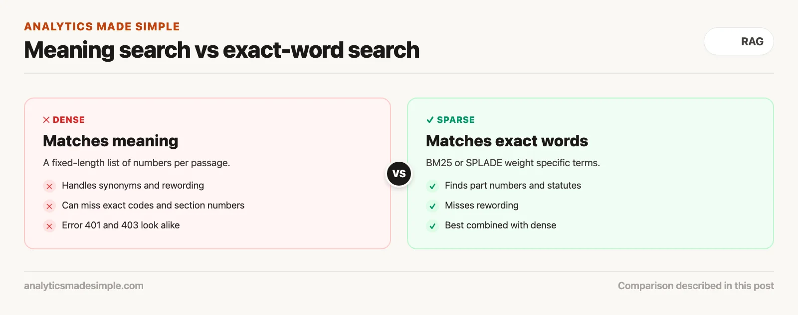
A sparse vector does the opposite. BM25 is one kind. SPLADE (a sparse model that also adds related words) is another. The vector has one slot per word in a big list, often 30,000 to 100,000 words. Only the words that are actually in the text get a weight. If the question contains 1798.100, that exact slot gets a heavy weight. If a document lacks that exact token, its score drops to zero. That is why sparse search catches exact words.

The 4 core embedding model archetypes

Modern RAG systems pick among four kinds of embedding model. Inference is the work a model does to produce an answer. The four kinds are small models that run fast on a normal chip (CPU), open models you host yourself, paid web APIs, and sparse models that catch exact words.

When you pick an embedding model, do not just take the one that ranks highest on the Massive Text Embedding Benchmark (MTEB). A benchmark is a standard test used to compare tools. Also look at the cost to run it, how much storage the numbers need, and how long an answer takes.

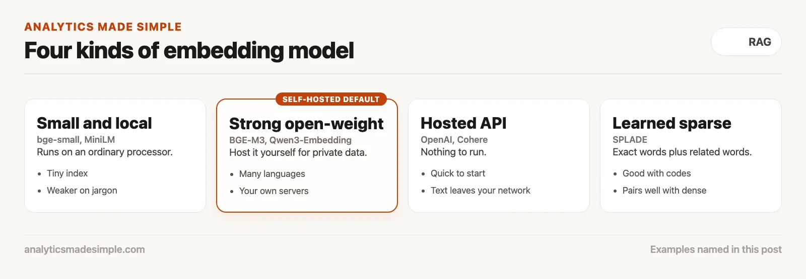
Here is how the four archetypes compare in production environments:

• 1. Lightweight edge models (e.g., BAAI/bge-small-en-v1.5, all-MiniLM-L6-v2): BAAI is short for the Beijing Academy of Artificial Intelligence. These small models make 384-number vectors. They run on a normal chip (CPU) in under 15 milliseconds. The vectors are small, so memory use stays low. They fit desktop apps, offline phone tools, and busy search when you have no graphics chip.
• 2. Strong open-weight models (e.g., BAAI/BGE-M3, Qwen3-Embedding, Nomic-Embed-Text): BGE is a family of embedding models from BAAI. These are the usual pick when you host the model yourself. BGE-M3 can make dense vectors, sparse word scores, and more than one vector in one pass. Its context window (how much text the AI can keep in view at once) holds 8,192 tokens, so you do not have to cut chunks short. Use them when you cannot send private text out. That includes the US law for patient data (HIPAA), the EU privacy law, and SOC 2, a common security audit (SOC is short for System and Organization Controls). HIPAA sets the rules for how patient data is handled.
• 3. Commercial managed APIs (e.g., OpenAI text-embedding-3, Cohere Embed v3): An API is a way for one program to ask another program for data or an action. These hosted tools make vectors of 1,536 to 3,072 numbers. You do not manage a graphics chip. They let you shorten the vector on the fly, which is called Matryoshka learning. In exchange, each call waits 100 to 200 milliseconds, you depend on their uptime, and you pay per token.
• 4. Learned sparse models (e.g., SPLADE): SPLADE sits between keyword search and deep learning. It does not output a fixed list of numbers. It adds related words to the question and writes a sparse weight for each word. You can store that in a normal search index such as Elasticsearch or OpenSearch. You do not need a special vector store.

Hybrid search in action: reciprocal rank fusion (RRF)

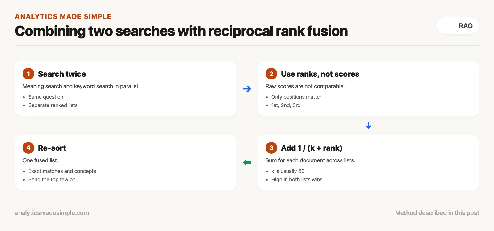
Reciprocal rank fusion combines the ranked candidate lists from dense vector search and sparse keyword search by adding up reciprocal rank positions. That way, documents that are strong in both meaning and exact wording rise to the top.

The gold standard for enterprise retrieval (looking up the relevant documents first) runs dense semantic search and sparse lexical search together in parallel, then fuses the results. That is harder than it sounds, because dense cosine similarities (floating-point numbers between 0.0 and 1.0) and BM25 scores (unbounded positive integers that can reach 45.0) live on completely different scales, so you cannot just add them together.

The industry solution is Reciprocal Rank Fusion (RRF). Instead of trying to normalize raw mathematical scores, RRF ignores the scores entirely and looks only at the rank order of the candidates. The formula is simple:

RRF_Score(d) = sum( 1.0 / (k + rank_i(d)) )

Where rank_i(d) is the position of document d in retrieval list i (1st place, 2nd place, and so on), and k is a smoothing constant (standardized at 60). A document that ranks 1st in dense search receives a score contribution of 1 / (60 + 1) = 0.01639. If that same document also ranks 2nd in BM25 keyword search, it receives an additional 1 / (60 + 2) = 0.01612, for a combined fusion score of 0.03251.

Here is a complete, dependency-free Python implementation showing how reciprocal rank fusion unites dense conceptual matches with sparse keyword matches:

def reciprocal_rank_fusion(
    dense_rankings: list[str],
    sparse_rankings: list[str],
    k: int = 60
) -> list[tuple[str, float]]:
    scores = {}

    # Process dense semantic rankings
    for rank, doc_id in enumerate(dense_rankings, 1):
        scores[doc_id] = scores.get(doc_id, 0.0) + (1.0 / (k + rank))

    # Process sparse lexical rankings
    for rank, doc_id in enumerate(sparse_rankings, 1):
        scores[doc_id] = scores.get(doc_id, 0.0) + (1.0 / (k + rank))

    sorted_results = sorted(scores.items(), key=lambda x: x[1], reverse=True)
    return sorted_results

# Query: "Requirements for third-party business disclosures under Cal. Civ. Code § 1798.100"
# Dense semantic search results (finds general privacy concepts)
dense_results = [
    "Doc_A: Consumer Privacy Rights Overview",
    "Doc_B: Third-Party Data Sharing Guidelines",
    "Doc_C: California Civ Code Section 1798.100 Statute",
    "Doc_D: GDPR International Transfer Rules"
]

# Sparse BM25 search results (finds exact alphanumeric statute matches)
sparse_results = [
    "Doc_C: California Civ Code Section 1798.100 Statute",
    "Doc_E: California Civil Code Historical Archive",
    "Doc_B: Third-Party Data Sharing Guidelines",
    "Doc_F: State Regulatory Disclosure Index"
]

fused_rankings = reciprocal_rank_fusion(dense_results, sparse_results, k=60)

print(f"{'Document ID':<45} | {'RRF Score':<12} | {'Rank'}")
print("-" * 65)
for pos, (doc, score) in enumerate(fused_rankings, 1):
    print(f"{doc:<45} | {score:.5f}    | #{pos}")

When you run this script, notice how the exact statute document (Doc_C) and the policy guidelines (Doc_B) rise to the absolute top of the rankings because they appear on both lists. Below is the rendered execution table:

Matryoshka representation learning: slashing vector storage by 80%

Matryoshka learning trains a model so the most useful signal sits in the front of the vector. You can cut a 3,072-number vector down to 512 numbers without training again. Storage and working memory (RAM) drop by more than 80 percent.

As libraries grow to millions of chunks, storage becomes a real limit. A chunk is one piece of a document that you store and search. A database of 5 million vectors, each 3,072 numbers long, uses over 60 gigabytes of memory (RAM) just to keep the index in memory for fast comparisons.

In the past, shortening a vector meant training a new model, or squeezing it afterward with a method called Principal Component Analysis (PCA). Modern models, including OpenAI text-embedding-3 and Nomic Embed, use Matryoshka Representation Learning (MRL) instead. The name comes from nested Russian dolls.

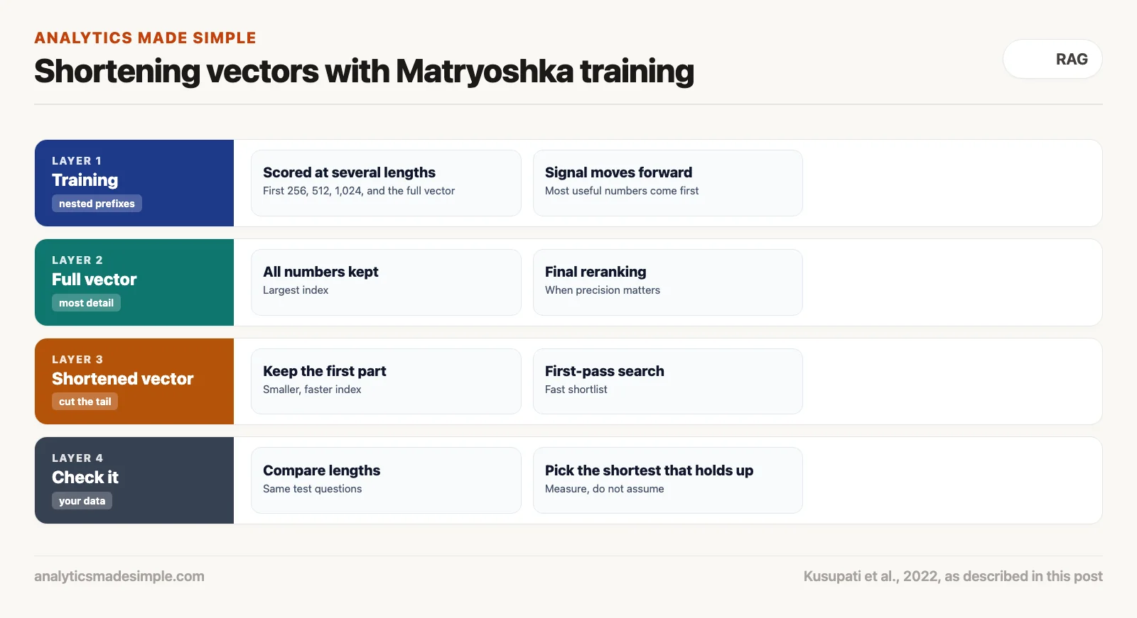
During training, the model is scored on nested prefixes: the first 256 numbers, the first 512, the first 1,024, and the full vector. That pushes the most useful signal to the front. At index time you can cut the vector with vector[:512] and scale it again. Cutting from 3,072 to 512 numbers shrinks vector memory by about 83 percent. Some search quality is lost, usually a little. In OpenAI’s January 2024 announcement, its large model cut down to just 256 numbers still beat its older full-size model on a standard search test (checked September 2026). Measure the loss on your own documents before you commit.

Practical rules for picking your embedding model on Monday

If you are building a cloud prototype, default to OpenAI text-embedding-3-small or Cohere Embed v3. If you are working under data privacy or on-premises constraints, self-host BAAI/BGE-M3 or Qwen3-Embedding with hybrid search instead.

When selecting your embedding model this week, follow this rubric:

• If you are a cloud-native startup: Start with OpenAI text-embedding-3-small or Cohere Embed v3. They provide reliable multi-lingual quality with zero infrastructure maintenance. Truncate dimensions to 512 using Matryoshka learning to keep the costs of the search database minimal.
• If you handle regulated health, financial, or private customer records: Deploy BAAI/BGE-M3 using vLLM or Text Embeddings Inference (TEI) on your own private graphics-chip servers. It provides data boundaries you control, multi-lingual coverage, and native sparse token generation.
• If you are searching code repositories or medical terminology: Implement hybrid search immediately. Pair your dense model with BM25 or SPLADE and fuse the rankings using reciprocal rank fusion (k=60). Never deploy a dense-only RAG system for legal or engineering documentation.
• If you are indexing documents longer than single paragraphs: Verify that your model supports at least an 8,192-token context window. Legacy models capped at 512 tokens silently truncate your text, dropping the second half of your chunk without warning.

The next post in this series covers metadata filtering: how tags, time-based rules, and per-tenant access rules keep vector search from returning documents a user should not see, or content that has gone out of date.

Sources and reference reading

• Muennighoff, N., et al, 2022, MTEB: Massive Text Embedding Benchmark, Proceedings of the 17th Conference of the EACL, https://arxiv.org/abs/2210.07316
• Chen, J., et al, 2024, BGE M3-Embedding: Multi-Lingual, Multi-Functionality, Multi-Granularity Text Embeddings Through Self-Knowledge Distillation, arXiv preprint, https://arxiv.org/abs/2402.03216
• Kusupati, A., et al, 2022, Matryoshka Representation Learning, Advances in Neural Information Processing Systems (NeurIPS), https://arxiv.org/abs/2205.13147
• Cormack, G. V., et al, 2009, Reciprocal Rank Fusion Outperforms Condorcet and Individual Rank Learning Methods, Proceedings of the 32nd International ACM SIGIR Conference, https://dl.acm.org/doi/10.1145/1571941.1572114
• Pinecone, Getting Started with Hybrid Search, Pinecone Learn (checked September 2026), https://www.pinecone.io/learn/hybrid-search-intro/

Series notes

This is Part 3 of RAG from scratch. Previous: chunking. Next: metadata filtering.

More definitions in Key Terms →

Merch on Etsy

Open store →

Standard Deviation T-Shirt View on Etsy → Apache Flink Shirt View on Etsy → Standard Deviation White Ceramic Mug View on Etsy → Mean Squared Error Shirt View on Etsy →